🔬Technical Deep Dive
Full Specifications [+]
Quick Commands
git clone https://github.com/FareedKhan-dev/autonomous-agentic-rag git clone https://github.com/FareedKhan-dev/autonomous-agentic-rag ⚖️ Nexus Index V16.5
💬 Index Insight
The Free2AITools Nexus Index for Autonomous Agentic Rag aggregates Popularity (P:0), Freshness (F:0), and Completeness (C:0). The Utility score (U:0) represents deployment readiness and ecosystem adoption.
Verification Authority
📋 Specs
- Language
- Jupyter Notebook
- License
- Open Source
- Version
- 1.0.0
Usage documentation not yet indexed for this tool.
🔗 View Source Code ↗Technical Documentation
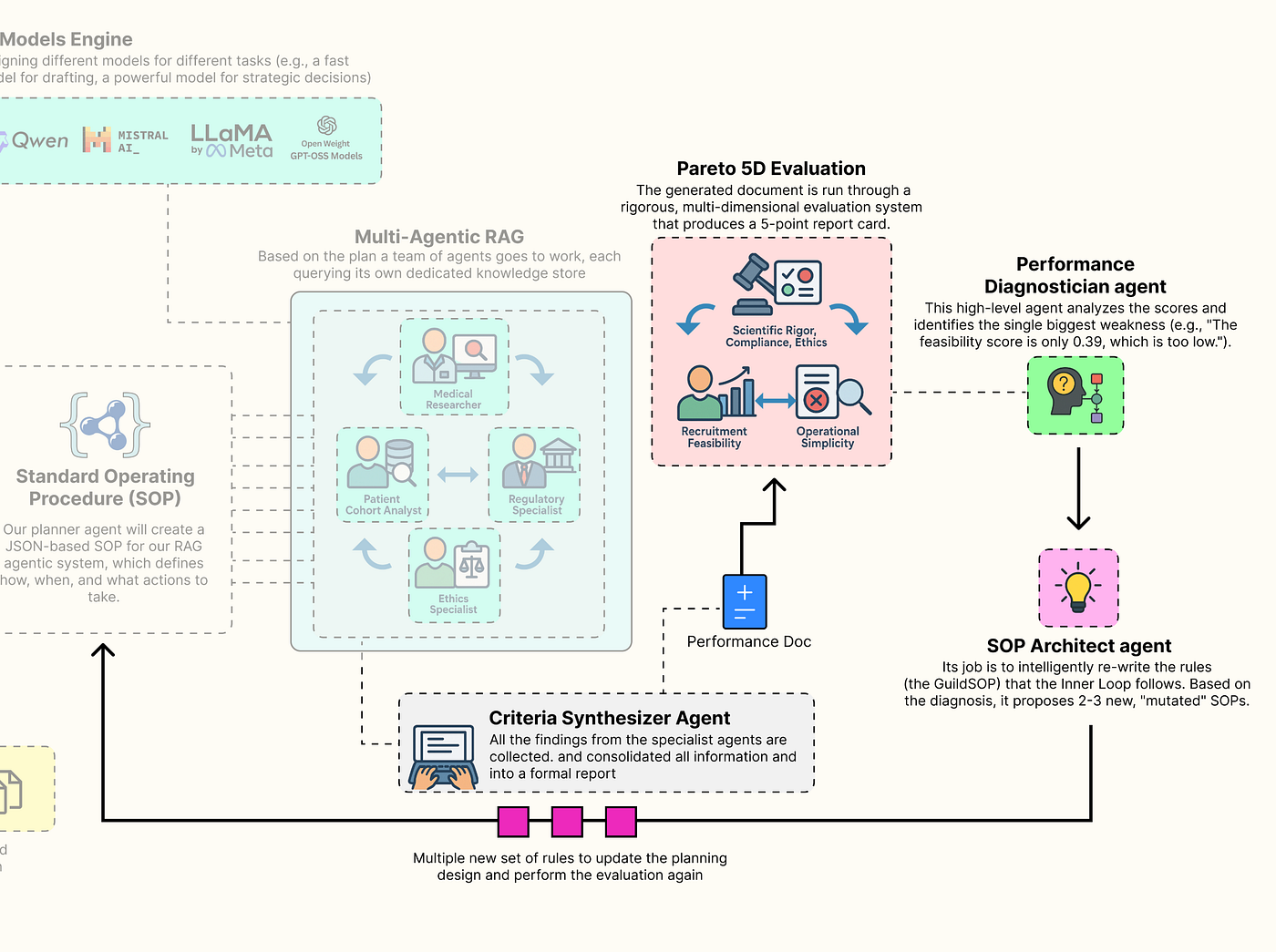
Building Self Improving RAG Agentic System
Agentic RAG systems act as a high dimensional vector space where each dimension represents a design decision such as prompt engineering, agent coordination, retrieval strategies, and much more. Manually tuning these dimensions to find the right combination is extremely difficult and unseen data in production often breaks what worked in testing.
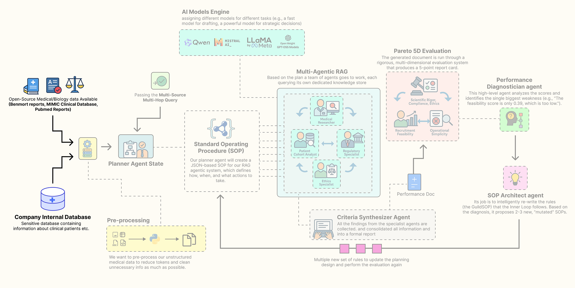
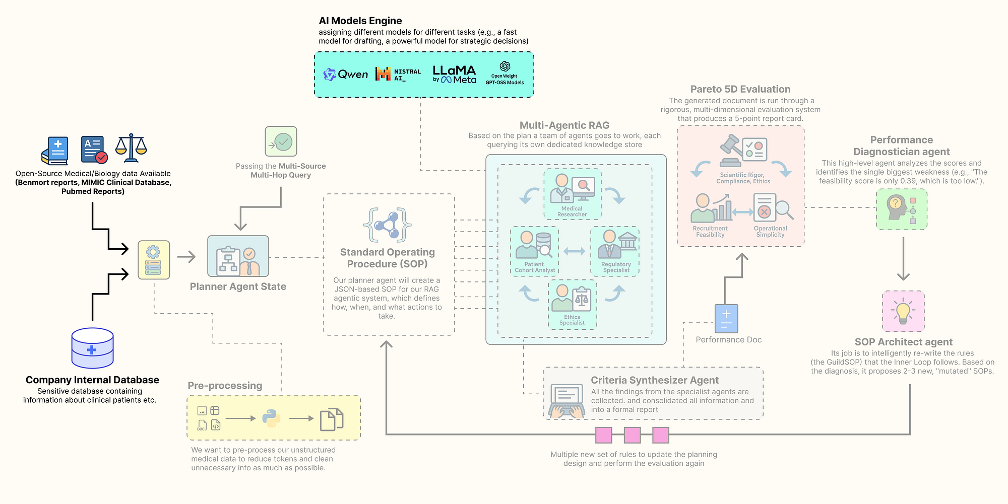
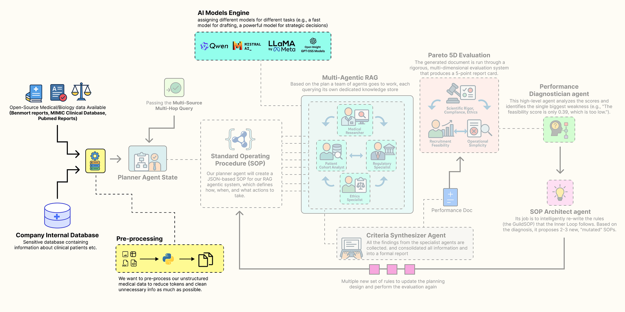
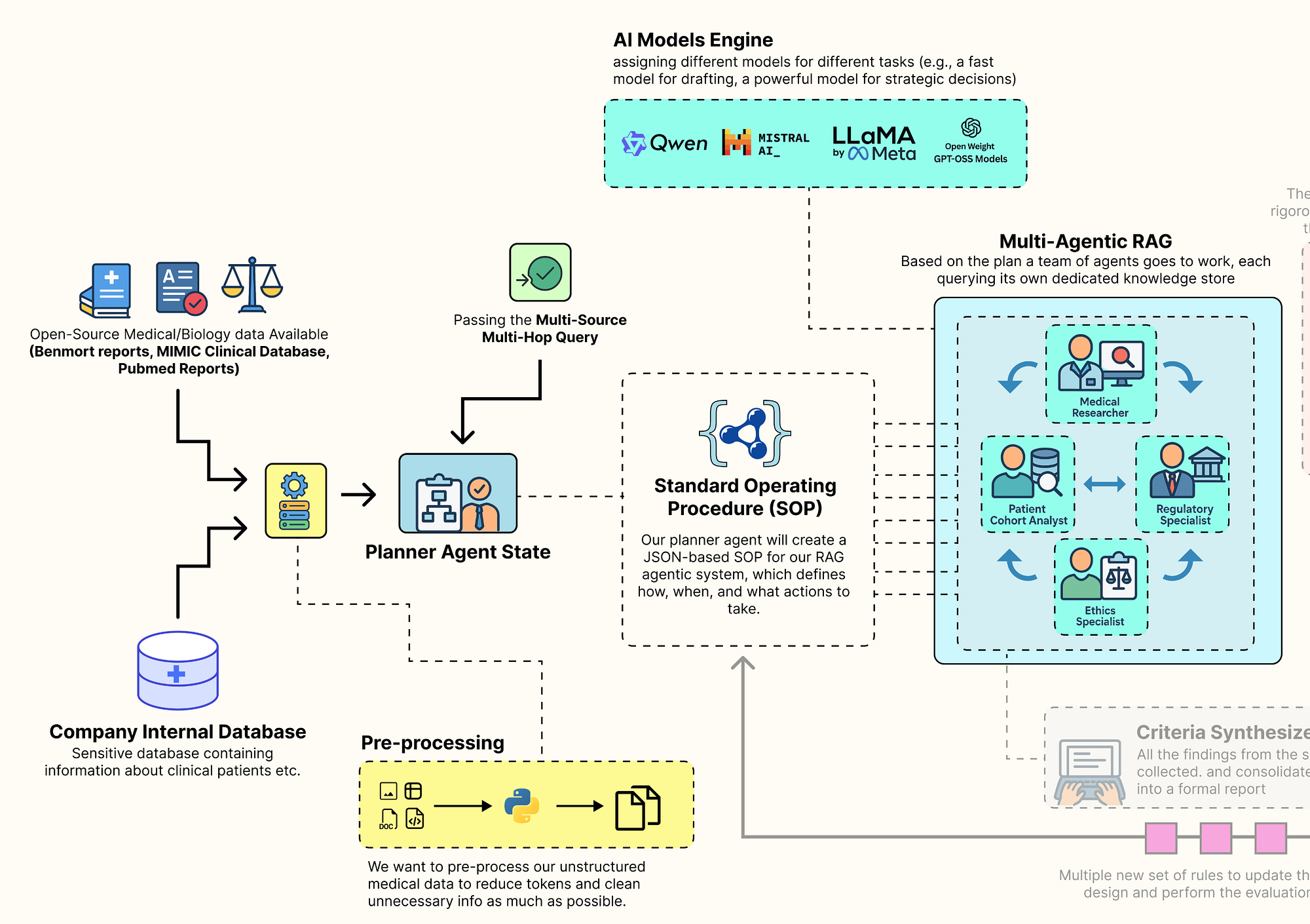
A better approach is to let the system learn how to optimize itself. A typical Agentic RAG pipeline that evolves itself follows the thinking process as shown below:
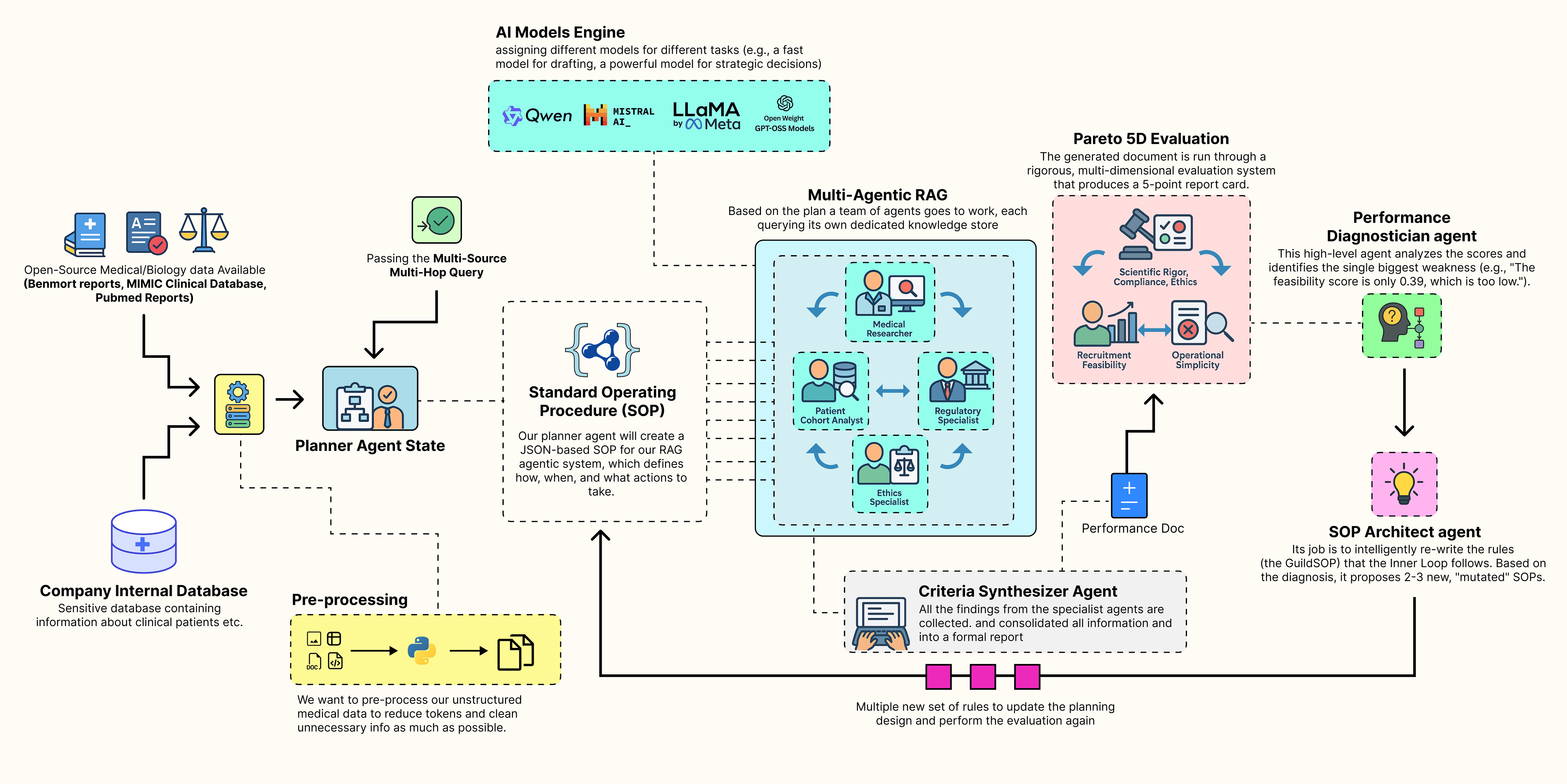 Self Improving Agentic RAG System (Created by Fareed Khan)
- A collaborative team of specialist agents carries out the task. It takes a high-level concept and generates a complete, multi-source document using its current standard operating procedures.
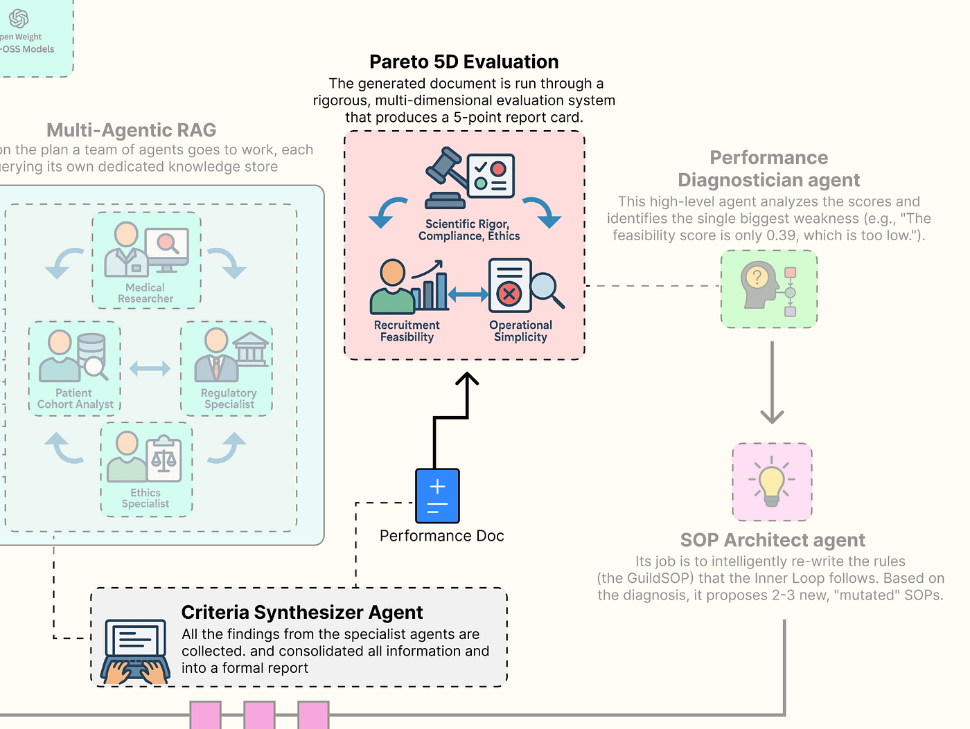
- A multi-dimensional evaluation system scores the team output, measuring performance across multiple goals such as accuracy, feasibility, and compliance, producing a performance vector.
- A performance diagnostician agent analyzes this vector, acting like a consultant to identify the main weakness in the process and trace its root cause.
- An SOP architect agent uses this insight to update the procedures, proposing new variations specifically designed to fix the identified weakness.
- Each new version of the SOP is tested as the team repeats the task, with each output evaluated again to produce its own performance vector.
- The system identifies the Pareto front, the best trade-offs among all tested SOPs and presents these optimized strategies to a human decision maker, completing the evolutionary loop.
In this blog, we are going to target the healthcare domain, which is very challenging because multiple possibilities need to be considered based on the input query or the knowledge base, while the final decision remains in the hands of a human.
We will build a complete end-to-end, self-improving Agentic RAG pipeline that generates different design patterns for RAG systems.
Table of Contents
- Knowledge Infrastructure for Medical AI
- Building The Inner Trial Design Network
- Multi-Dimensional Evaluation System
- Outer Loop of the Evolution Engine
- 5D Pareto Based Analysis
- Understanding the Cognitive Workflow
- Making it an Autonomous Strategy
Knowledge Infrastructure for Medical AI
Before we can code our self-evolving agentic RAG system, we need to establish a proper knowledge database along with the necessary tools required to build the architecture.
A production-grade RAG system typically contains a diverse set of databases, including sensitive organizational data as well as open-source data, to improve retrieval quality and compensate for outdated or incomplete information. This foundational step is arguably the most critical …
as the quality of our data sources will directly determine the quality of our final output.
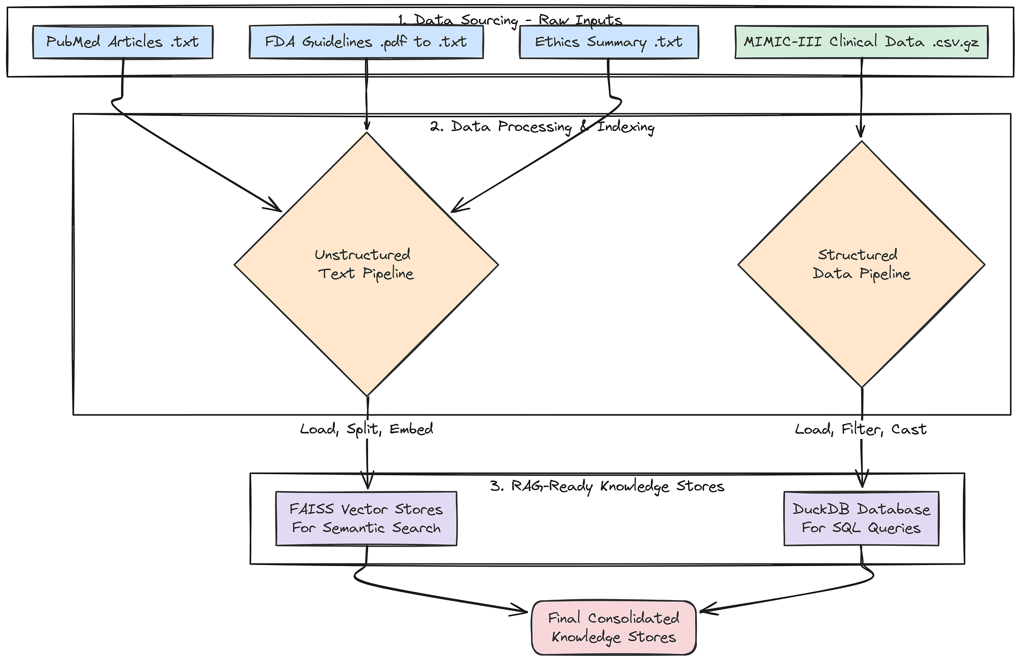
 Sourcing the knowledge base (Created by Fareed Khan)
In this section, we are going to assemble every component of this architecture. Here is what we are going to do:
- Install the Open-Source Stack: We will set up our environment with all the necessary libraries, focusing on a local, open-source-first approach.
- Configure Secure Observability: Then going to securely load our API keys and configure
LangSmithto trace and debug our complex agent interactions from the very beginning. - Build a Local LLM Foundry: We are going to build a suite of different open-source models using
Ollama, assigning specific models to specific tasks to optimize for performance and cost. - Source and Process Multi-Modal Data: downloading and preparing four real-world data sources: scientific literature from PubMed, regulatory guidelines from the FDA, ethical principles, and a massive structured clinical dataset (MIMIC-III).
- Index the Knowledge Stores: Finally, we will process this raw data into highly efficient, searchable databases,
FAISSvector stores for our unstructured text and aDuckDBinstance for our structured clinical data.
Installing the Open-Source Stack
So, our first step is to install all the required Python libraries. A reproducible environment is the bedrock of any serious project. We are selecting a industry-standard, open-source stack that gives us full control over our system. This includes langchain and langgraph for the core agentic framework, ollama for interacting with our local LLMs, and specialized libraries like biopython for accessing PubMed and duckdb for high-performance analytics on our clinical data.
Let’s install the required modules …
# We uses pip "quiet" (-q) and "upgrade" (-U) flags to install all the required packages.
# - langchain, langgraph, etc.: These form the core of our agentic framework for building and orchestrating agents.
# - ollama: This is the client library that allows our Python code to communicate with a locally running Ollama server.
# - duckdb: An incredibly fast, in-process analytical database perfect for handling our structured MIMIC data without a heavy server setup.
# - faiss-cpu: Facebook AI's library for efficient similarity search, which will power the vector stores for our RAG agents.
# - sentence-transformers: A library for easy access to state-of-the-art models for creating text embeddings.
# - biopython, pypdf, beautifulsoup4: A suite of powerful utilities for downloading and parsing our diverse, real-world data sources.
%pip install -U langchain langgraph langchain_community langchain_openai langchain_core ollama pandas duckdb faiss-cpu sentence-transformers biopython pypdf pydantic lxml html2text beautifulsoup4 matplotlib -qqq
We are gathering all the tools and building materials we will need for the rest of the project in one go. Each library has a specific role, from agent workflows with langgraph to data analysis with duckdb.
Now that w have installed the required modules, let’s start initializing them one by one.
Environment Configuration & Imports
We need to securely configure our environment. Hardcoding API keys directly into a notebook is a significant security risk and makes the code difficult to share.
We will use a .env file to manage our secrets, primarily our LangSmith API key. Setting up LangSmith from the very beginning is non-negotiable for a project of this complexity, it provides the deep observability we will need to trace, debug, and understand the interactions between our agents. So, let’s do that.
import os
import getpass
from dotenv import load_dotenv

# This function from the python-dotenv library searches for a .env file and loads its key-value pairs
# into the operating system's environment variables, making them accessible to our script.
load_dotenv()

# This is a critical check. We verify that our script can access the necessary API keys from the environment.
if "LANGCHAIN_API_KEY" not in os.environ or "ENTREZ_EMAIL" not in os.environ:
    # If the keys are missing, we print an error and halt, as the application cannot proceed.
    print("Required environment variables not set. Please set them in your .env file or environment.")
else:
    # This confirmation tells us our secrets have been loaded securely and are ready for use.
    print("Environment variables loaded successfully.")

# We explicitly set the LangSmith project name. This is a best practice that ensures all traces

# generated by this project are automatically grouped together in the LangSmith user interface for easy analysis.
os.environ["LANGCHAIN_PROJECT"] = "AI_Clinical_Trials_Architect"
The function load_dotenv() acts as a secure bridge between our sensitive credentials and our code. It reads the .env file (which should never be committed to version control) and injects the keys into our session environment.
From this point forward, every operation we perform with LangChain or LangGraph will be automatically captured and sent to our project in LangSmith.
Configuring the Local LLM
In production-grade agentic systems, a one-size-fits-all model strategy is rarely optimal. A massive, state-of-the-art model is computationally expensive and slow, using it for every simple task would be waste of resources especially if it’s hosted on your GPUs. But a small, fast model might lack the deep reasoning power needed for high-stakes strategic decisions.
 Configuring Local LLMs (Created by Fareed Khan)
The key is to fit the right model at right place of your agentic system. We will build a group of different open-source models, each chosen for its strengths in a specific role, and all served locally via Ollama for privacy, control, and cost-effectiveness.
We need to define a configuration dictionary to hold the clients for each of our chosen models. This way we can easily swap models and centralizes our model management.
from langchain_community.chat_models import ChatOllama
from langchain_community.embeddings import OllamaEmbeddings

# This dictionary will act as our central registry, or "foundry," for all LLM and embedding model clients.
llm_config = {
    # For the 'planner', we use Llama 3.1 8B. It's a modern, highly capable model that excels at instruction-following.
    # We set `format='json'` to leverage Ollama's built-in JSON mode, ensuring reliable structured output for this critical task.
    "planner": ChatOllama(model="llama3.1:8b-instruct", temperature=0.0, format='json'),

    # For the 'drafter' and 'sql_coder', we use Qwen2 7B. It's a nimble and fast model, perfect for
    # tasks like text generation and code completion where speed is valuable.
    "drafter": ChatOllama(model="qwen2:7b", temperature=0.2),
    "sql_coder": ChatOllama(model="qwen2:7b", temperature=0.0),

    # For the 'director', the highest-level strategic agent, we use the powerful Llama 3 70B model.
    # This high-stakes task of diagnosing performance and evolving the system's own procedures
    # justifies the use of a larger, more powerful model.
    "director": ChatOllama(model="llama3:70b", temperature=0.0, format='json'),
    # For embeddings, we use 'nomic-embed-text', a top-tier, efficient open-source model.
    "embedding_model": OllamaEmbeddings(model="nomic-embed-text")
}
So we have just created our llm_config dictionary, which serves as a centralized hub for all our model initializations. By assigning different models to different roles, we are creating a cost-performance optimized hierarchy.
- Fast & Nimble (7B-8B models): The
planner,drafter, andsql_coderroles handle frequent, well-defined tasks. Using smaller models likeQwen2 7BandLlama 3.1 8Bfor these roles ensures low latency and efficient resource usage. They are perfectly capable of following instructions to generate plans, draft text, or write SQL. - Deep & Strategic (70B model): The
directoragent has the most complex job, it must analyze multi-dimensional performance data and rewrite the entire system operating procedure. This requires deep reasoning and a understanding of cause and effect. For this high-stakes, low-frequency task, we allocate our most powerful resource, theLlama 3 70Bmodel.
Let’s execute this cell to initialize the clients and print their configurations.
# Print the configuration to confirm the clients are initialized and their parameters are set correctly.
print("LLM clients configured:")
print(f"Planner ({llm_config['planner'].model}): {llm_config['planner']}")
print(f"Drafter ({llm_config['drafter'].model}): {llm_config['drafter']}")
print(f"SQL Coder ({llm_config['sql_coder'].model}): {llm_config['sql_coder']}")
print(f"Director ({llm_config['director'].model}): {llm_config['director']}")
print(f"Embedding Model ({llm_config['embedding_model'].model}): {llm_config['embedding_model']}")
This is what we are getting …
#### OUTPUT ####
LLM clients configured:
Planner (llama3.1:8b-instruct): ChatOllama(model='llama3.1:8b-instruct', temperature=0.0, format='json')
Drafter (qwen2:7b): ChatOllama(model='qwen2:7b', temperature=0.2)
SQL Coder (qwen2:7b): ChatOllama(model='qwen2:7b', temperature=0.0)
Director (llama3:70b): ChatOllama(model='llama3:70b', temperature=0.0, format='json')
Embedding Model (nomic-embed-text): OllamaEmbeddings(model='nomic-embed-text')
The output confirms that our ChatOllama and OllamaEmbeddings clients have been successfully initialized with their respective models and parameters. now we are ready to be connected with our knowledge stores.
Preparing the Knowledge Stores
RAG most important part is this, a rich multi-modal knowledge base to draw upon. A generic, web-based search is not enough for a specialized task like clinical trial design. We need to ground our agents in authoritative, domain-specific information.
 Knowledge store creation (Created by Fareed Khan)
To achieve this, we will now build a comprehensive knowledge base by sourcing, downloading, and processing four distinct types of real-world data. This multi-source approach is critical for enabling our agents to synthesize information and produce a comprehensive, well-rounded output.
First, a small but important step: we will create the directories where our downloaded and processed data will live.
import os

# A dictionary to hold the paths for our different data types. This keeps our file management clean and centralized.
data_paths = {
    "base": "./data",
    "pubmed": "./data/pubmed_articles",
    "fda": "./data/fda_guidelines",
    "ethics": "./data/ethical_guidelines",
    "mimic": "./data/mimic_db"
}
# This loop iterates through our defined paths and uses os.makedirs() to create any directories that don't already exist.
# This prevents errors in later steps when we try to save files to these locations.
for path in data_paths.values():
    if not os.path.exists(path):
        os.makedirs(path)
        print(f"Created directory: {path}")
We are making sure our project has a clean and organized file structure from the start. By pre-defining and creating these directories, our subsequent data processing functions become more robust, they can reliably save their outputs to the correct location without needing to check if the directory exists first.
Next, we will fetch real scientific literature from PubMed. This will provide the core knowledge for our Medical Researcher agent, grounding its work in up-to-date, peer-reviewed science.
from Bio import Entrez
from Bio import Medline

def download_pubmed_articles(query, max_articles=20):
    """Fetches abstracts from PubMed for a given query and saves them as text files."""
    # The NCBI API requires an email address for identification. We fetch it from our environment variables.
    Entrez.email = os.environ.get("ENTREZ_EMAIL")
    print(f"Fetching PubMed articles for query: {query}")

    # Step 1: Use Entrez.esearch to find the PubMed IDs (PMIDs) for articles matching our query.
    handle = Entrez.esearch(db="pubmed", term=query, retmax=max_articles, sort="relevance")
    record = Entrez.read(handle)
    id_list = record["IdList"]
    print(f"Found {len(id_list)} article IDs.")

    print("Downloading articles...")
    # Step 2: Use Entrez.efetch to retrieve the full records (in MEDLINE format) for the list of PMIDs.
    handle = Entrez.efetch(db="pubmed", id=id_list, rettype="medline", retmode="text")
    records = Medline.parse(handle)

    count = 0
    # Step 3: Iterate through the retrieved records, parse them, and save each abstract to a file.
    for i, record in enumerate(records):
        pmid = record.get("PMID", "")
        title = record.get("TI", "No Title")
        abstract = record.get("AB", "No Abstract")
        if pmid:
            # We name the file after the PMID for easy reference and to avoid duplicates.
            filepath = os.path.join(data_paths["pubmed"], f"{pmid}.txt")
            with open(filepath, "w") as f:
                f.write(f"Title: {title}\n\nAbstract: {abstract}")
            print(f"[{i+1}/{len(id_list)}] Fetching PMID: {pmid}... Saved to {filepath}")
            count += 1
    return count
The download_pubmed_articles function is our direct connection to the live scientific literature. It's a three-step process:
esearchto find relevant article IDs,efetchto download the full records.- Then a loop to parse and save the crucial information (Title and Abstract) into clean text files.
Let’s run this function with a query specific to our use case.
# We define a specific, boolean query to find articles highly relevant to our trial concept.
pubmed_query = "(SGLT2 inhibitor) AND (type 2 diabetes) AND (renal impairment)"
num_downloaded = download_pubmed_articles(pubmed_query)
print(f"PubMed download complete. {num_downloaded} articles saved.")
When we run the above code, it will start downloading the pubmed articles highly relevant to our query.
#### OUTPUT ####
Fetching PubMed articles for query: (SGLT2 inhibitor) AND (type 2 diabetes) AND (renal impairment)
Found 20 article IDs.
Downloading articles...
[1/20] Fetching PMID: 38810260... Saved to ./data/pubmed_articles/38810260.txt
[2/20] Fetching PMID: 38788484... Saved to ./data/pubmed_articles/38788484.txt
...
PubMed download complete. 20 articles saved.
It successfully connected to the NCBI database, executed our specific query, and downloaded 20 relevant scientific abstracts, saving each one into our designated pubmed_articles directory.
Our Medical Researcher agent will now has a rich, current, and domain-specific knowledge base to draw from, ensuring its findings are grounded in real science.
Now, let’s get the regulatory documents that our Regulatory Specialist agent will need. A key part of trial design is ensuring compliance with government guidelines.
import requests
from pypdf import PdfReader
import io

def download_and_extract_text_from_pdf(url, output_path):
    """Downloads a PDF from a URL, saves it, and also extracts its text content to a separate .txt file."""
    print(f"Downloading FDA Guideline: {url}")
    try:
        # We use the 'requests' library to perform the HTTP GET request to download the file.
        response = requests.get(url)
        response.raise_for_status() # This is a good practice that will raise an error if the download fails (e.g., a 404 error).

        # We save the raw PDF file, which is useful for archival purposes.
        with open(output_path, 'wb') as f:
            f.write(response.content)
        print(f"Successfully downloaded and saved to {output_path}")

        # We then use pypdf to read the PDF content directly from the in-memory response.
        reader = PdfReader(io.BytesIO(response.content))
        text = ""
        # We loop through each page of the PDF and append its extracted text.
        for page in reader.pages:
            text += page.extract_text() + "\n\n"

        # Finally, we save the clean, extracted text to a .txt file. This is the file our RAG system will actually use.
        txt_output_path = os.path.splitext(output_path)[0] + '.txt'
        with open(txt_output_path, 'w') as f:
            f.write(text)
        return True
    except requests.exceptions.RequestException as e:
        print(f"Error downloading file: {e}")
        return False
This function, download_and_extract_text_from_pdf, is our tool for handling PDF documents. It's a two-stage process.
- First, it downloads and saves the original PDF from the FDA website. Second, and more importantly, it immediately processes that PDF using
pypdfto extract all the text content. - It then saves this raw text to a
.txtfile. This pre-processing step is crucial because it converts the complex PDF format into simple text that our document loaders can easily ingest when we build our vector stores later on.
Let’s run the function to download our FDA guidance document.
# This URL points to a real FDA guidance document for developing drugs for diabetes.
fda_url = "https://www.fda.gov/media/71185/download"
fda_pdf_path = os.path.join(data_paths["fda"], "fda_diabetes_guidance.pdf")
download_and_extract_text_from_pdf(fda_url, fda_pdf_path)

#### OUTPUT ####
Downloading FDA Guideline: https://www.fda.gov/media/71185/download
Successfully downloaded and saved to ./data/fda_guidelines/fda_diabetes_guidance.pdf
We now have both the original fda_diabetes_guidance.pdf and its extracted text version in our fda_guidelines directory. Our Regulatory Specialist agent is now equipped with its foundational legal and regulatory text.
Next, we will create a curated document for our Ethics Specialist. While we could search for this information, providing a concise, authoritative summary of core principles ensures the agent's reasoning is grounded in the most important concepts.
# This multi-line string contains a curated summary of the three core principles of the Belmont Report,
# which is the foundational document for ethics in human subject research in the United States.
ethics_content = """
Title: Summary of the Belmont Report Principles for Clinical Research
1. Respect for Persons: This principle requires that individuals be treated as autonomous agents and that persons with diminished autonomy are entitled to protection. This translates to robust informed consent processes. Inclusion/exclusion criteria must not unduly target or coerce vulnerable populations, such as economically disadvantaged individuals, prisoners, or those with severe cognitive impairments, unless the research is directly intended to benefit that population.
2. Beneficence: This principle involves two complementary rules: (1) do not harm and (2) maximize possible benefits and minimize possible harms. The criteria must be designed to select a population that is most likely to benefit and least likely to be harmed by the intervention. The risks to subjects must be reasonable in relation to anticipated benefits.
3. Justice: This principle concerns the fairness of distribution of the burdens and benefits of research. The selection of research subjects must be equitable. Criteria should not be designed to exclude certain groups without a sound scientific or safety-related justification. For example, excluding participants based on race, gender, or socioeconomic status is unjust unless there is a clear rationale related to the drug's mechanism or risk profile.
"""

# We define the path where our ethics document will be saved.
ethics_path = os.path.join(data_paths["ethics"], "belmont_summary.txt")

# We open the file in write mode and save the content.
with open(ethics_path, "w") as f:
    f.write(ethics_content)
print(f"Created ethics guideline file: {ethics_path}")
We have created a focused document for our Ethics Specialist. Instead of having the agent sift through the entire Belmont Report, we have provided it with the most critical information in a clean, easily digestible format. This ensures its analysis will be consistent and grounded in the core principles.
Now for our most complex data source: the structured clinical data from MIMIC-III. This will provide the real-world population data our Patient Cohort Analyst needs to assess recruitment feasibility.
import duckdb
import pandas as pd
import os


def load_real_mimic_data():
    """Loads real MIMIC-III CSVs into a persistent DuckDB database file, processing the massive LABEVENTS table efficiently."""
    print("Attempting to load real MIMIC-III data from local CSVs...")
    db_path = os.path.join(data_paths["mimic"], "mimic3_real.db")
    csv_dir = os.path.join(data_paths["mimic"], "mimiciii_csvs")

    # Define the paths to the required compressed CSV files.
    required_files = {
        "patients": os.path.join(csv_dir, "PATIENTS.csv.gz"),
        "diagnoses": os.path.join(csv_dir, "DIAGNOSES_ICD.csv.gz"),
        "labevents": os.path.join(csv_dir, "LABEVENTS.csv.gz"),
    }

    # Before starting, we check if all the necessary source files are present.
    missing_files = [path for path in required_files.values() if not os.path.exists(path)]
    if missing_files:
        print("ERROR: The following MIMIC-III files were not found:")
        for f in missing_files: print(f"- {f}")
        print("\nPlease download them as instructed and place them in the correct directory.")
        return None

    print("Required files found. Proceeding with database creation.")
    # Remove any old database file to ensure we are building from scratch.
    if os.path.exists(db_path):
        os.remove(db_path)
    # Connect to DuckDB. If the database file doesn't exist, it will be created.
    con = duckdb.connect(db_path)

    # Use DuckDB's powerful `read_csv_auto` to directly load data from the gzipped CSVs into SQL tables.
    print(f"Loading {required_files['patients']} into DuckDB...")
    con.execute(f"CREATE TABLE patients AS SELECT SUBJECT_ID, GENDER, DOB, DOD FROM read_csv_auto('{required_files['patients']}')")

    print(f"Loading {required_files['diagnoses']} into DuckDB...")
    con.execute(f"CREATE TABLE diagnoses_icd AS SELECT SUBJECT_ID, ICD9_CODE FROM read_csv_auto('{required_files['diagnoses']}')")

    # The LABEVENTS table is enormous. To handle it robustly, we use a two-stage process.
    print(f"Loading and processing {required_files['labevents']} (this may take several minutes)...")
    # 1. Load the data into a temporary 'staging' table, treating all columns as text (`all_varchar=True`).
    #    This prevents parsing errors with mixed data types. We also filter for only the lab item IDs we
    #    care about (50912 for Creatinine, 50852 for HbA1c) and use a regex to ensure VALUENUM is numeric.
    con.execute(f"""CREATE TABLE labevents_staging AS
                   SELECT SUBJECT_ID, ITEMID, VALUENUM
                   FROM read_csv_auto('{required_files['labevents']}', all_varchar=True)
                   WHERE ITEMID IN ('50912', '50852') AND VALUENUM IS NOT NULL AND VALUENUM ~ '^[0-9]+(\\.[0-9]+)?$'
                """)
    # 2. Create the final, clean table by selecting from the staging table and casting the columns to their correct numeric types.
    con.execute("CREATE TABLE labevents AS SELECT SUBJECT_ID, CAST(ITEMID AS INTEGER) AS ITEMID, CAST(VALUENUM AS DOUBLE) AS VALUENUM FROM labevents_staging")
    # 3. Drop the temporary staging table to save space.
    con.execute("DROP TABLE labevents_staging")
    con.close()
    return db_path
Instead of trying to load the massive MIMIC-III CSV files into memory with pandas (which would likely crash), we are usingDuckDB ability to process data directly from disk. The two-stage processing of theLABEVENTS table is a critical technique. By first loading the data as text and filtering it before casting to numeric types, before this we handle data quality issues and create a final table that is smaller, cleaner, and much faster to query.
Let’s execute the function to build our clinical database and then run a quick test to inspect the result.
# Execute the function to build the database.
db_path = load_real_mimic_data()

# If the database was created successfully, connect to it and inspect the schema and some sample data.
if db_path:
    print(f"\nReal MIMIC-III database created at: {db_path}")
    print("\nTesting database connection and schema...")
    con = duckdb.connect(db_path)
    print(f"Tables in DB: {con.execute('SHOW TABLES').df()['name'].tolist()}")
    print("\nSample of 'patients' table:")
    print(con.execute("SELECT * FROM patients LIMIT 5").df())
    print("\nSample of 'diagnoses_icd' table:")
    print(con.execute("SELECT * FROM diagnoses_icd LIMIT 5").df())
    con.close()
The output we are getting …
#### OUTPUT ####
Attempting to load real MIMIC-III data from local CSVs...
Required files found. Proceeding with database creation.
Loading PATIENTS.csv.gz into DuckDB...
Loading DIAGNOSES_ICD.csv.gz into DuckDB...
Loading and processing LABEVENTS.csv.gz (this may take several minutes)...

Real MIMIC-III database created at: ./data/mimic_db/mimic3_real.db
Testing database connection and schema...
Tables in DB: ['patients', 'diagnoses_icd', 'labevents']
Sample of 'patients' table:
   ROW_ID  SUBJECT_ID GENDER         DOB         DOD    DOD_HOSP    DOD_SSN EXPIRE_FLAG
0      238       250      F  2164-12-27  2198-02-18  2198-02-18 2198-02-18           1
1      239       251      M  2078-02-21         NaN         NaN        NaN           0
2      240       252      M  2049-06-06  2123-09-01  2123-09-01 2123-09-01           1
3      241       253      F  2081-11-26         NaN         NaN        NaN           0
4      242       254      F  2028-04-12         NaN         NaN        NaN           0

Sample of 'diagnoses_icd' table:
   ROW_ID  SUBJECT_ID  HADM_ID  SEQ_NUM ICD9_CODE
0  129769       109    172335        1      40301
1  129770       109    172335        2      486
2  129771       109    172335        3      58281
3  129772       109    172335        4      5855
4  129773       109    172335        5      42822
The output confirms that our data ingestion pipeline worked. We have successfully created a persistent DuckDB SQL database at ./data/mimic_db/mimic3_real.db. The test queries show that the core tables (patients, diagnoses_icd, labevents) have been loaded correctly with the right schemas.
Our Patient Cohort Analyst agent now has access to a high-performance, real-world clinical database containing millions of records, enabling it to provide truly data-grounded feasibility estimates.
 Pre-processing Step (Created by Fareed Khan)
Finally, let’s index all our unstructured text data into searchable vector stores. This will make the PubMed, FDA, and ethics documents accessible to our RAG agents.
from langchain_community.document_loaders import DirectoryLoader, TextLoader
from langchain.text_splitter import RecursiveCharacterTextSplitter
from langchain_community.vectorstores import FAISS
from langchain_core.documents import Document

def create_vector_store(folder_path: str, embedding_model, store_name: str):
    """Loads all .txt files from a folder, splits them into chunks, and creates an in-memory FAISS vector store."""
    print(f"--- Creating {store_name} Vector Store ---")
    # Use DirectoryLoader to efficiently load all .txt files from the specified folder.
    loader = DirectoryLoader(folder_path, glob="**/*.txt", loader_cls=TextLoader, show_progress=True)
    documents = loader.load()

    if not documents:
        print(f"No documents found in {folder_path}, skipping vector store creation.")
        return None

    # Use RecursiveCharacterTextSplitter to break large documents into smaller, 1000-character chunks with a 100-character overlap.
    # The overlap helps maintain context between chunks.
    text_splitter = RecursiveCharacterTextSplitter(chunk_size=1000, chunk_overlap=100)
    texts = text_splitter.split_documents(documents)

    print(f"Loaded {len(documents)} documents, split into {len(texts)} chunks.")
    print("Generating embeddings and indexing into FAISS... (This may take a moment)")
    # FAISS.from_documents is a convenient function that handles both embedding the text chunks
    # and building the efficient FAISS index in one step.
    db = FAISS.from_documents(texts, embedding_model)
    print(f"{store_name} Vector Store created successfully.")
    return db

def create_retrievers(embedding_model):
    """Creates vector store retrievers for all unstructured data sources and consolidates all knowledge stores."""
    # Create a separate, specialized vector store for each type of document.
    pubmed_db = create_vector_store(data_paths["pubmed"], embedding_model, "PubMed")
    fda_db = create_vector_store(data_paths["fda"], embedding_model, "FDA")
    ethics_db = create_vector_store(data_paths["ethics"], embedding_model, "Ethics")

    # Return a single dictionary containing all configured data access tools.
    # The 'as_retriever' method converts the vector store into a standard LangChain Retriever object.
    # The 'k' parameter in 'search_kwargs' controls how many top documents are returned by a search.
    return {
        "pubmed_retriever": pubmed_db.as_retriever(search_kwargs={"k": 3}) if pubmed_db else None,
        "fda_retriever": fda_db.as_retriever(search_kwargs={"k": 3}) if fda_db else None,
        "ethics_retriever": ethics_db.as_retriever(search_kwargs={"k": 2}) if ethics_db else None,
        "mimic_db_path": db_path # We also include the file path to our structured DuckDB database.
    }
This create_vector_store function is the approach for creating RAG-ready knowledge bases from text files. It encapsulates the common "load -> split -> embed -> index" pattern. The create_retrievers function then orchestrates this process, creating a separate, specialized vector store for each of our document types.
Instead of a single, massive vector store, we have smaller, domain-specific stores. This allows our agents to perform more targeted and efficient searches (e.g., the Regulatory Specialist will only ever query the fda_retriever).
Let’s run the final function to build our complete set of knowledge stores.
# Execute the function to create all our retrievers.
knowledge_stores = create_retrievers(llm_config["embedding_model"])

print("\nKnowledge stores and retrievers created successfully.")

# Print the final dictionary to confirm all components are present.
for name, store in knowledge_stores.items():
print(f"{name}: {store}")#### OUTPUT ####
--- Creating PubMed Vector Store ---
100%|██████████| 20/20 [00:00<00:00, 1102.77it/s]
Loaded 20 documents, split into 35 chunks.
Generating embeddings and indexing into FAISS... (This may take a moment)
Batches: 100%|██████████| 2/2 [00:03<00:00, 1.70s/it]
PubMed Vector Store created successfully.
--- Creating FDA Vector Store ---
100%|██████████| 1/1 [00:00<00:00, 137.95it/s]
Loaded 1 documents, split into 48 chunks.
Generating embeddings and indexing into FAISS... (This may take a moment)
Batches: 100%|██████████| 2/2 [00:04<00:00, 2.08s/it]
FDA Vector Store created successfully.
--- Creating Ethics Vector Store ---
100%|██████████| 1/1 [00:00<00:00, 143.20it/s]
Loaded 1 documents, split into 1 chunks.
Generating embeddings and indexing into FAISS... (This may take a moment)
Batches: 100%|██████████| 1/1 [00:00<00:00, 2.62it/s]
Ethics Vector Store created successfully.
Knowledge stores and retrievers created successfully.
pubmed_retriever: VectorStoreRetriever(tags=['FAISS', 'OllamaEmbeddings'], vectorstore=<...>)
fda_retriever: VectorStoreRetriever(tags=['FAISS', 'OllamaEmbeddings'], vectorstore=<...>)
ethics_retriever: VectorStoreRetriever(tags=['FAISS', 'OllamaEmbeddings'], vectorstore=<...>)
mimic_db_path: ./data/mimic_db/mimic3_real.dbThe output confirms that our entire knowledge is now fully assembled and operational. We have successfully processed all our unstructured text sources, PubMed, FDA, and Ethics into searchable FAISS vector stores.
The final knowledge_stores dictionary is our complete, centralized repository of data access tools. It contains everything our agent guild will need to perform its research.
With our data downloaded, processed, and indexed, and our LLMs configured, we can now begin constructing the first major component of our agentic system: The Trial Design Guild.
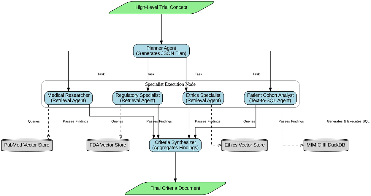
Building The Inner Trial Design Network
With our knowledge base is now ready, we can now construct the core of our system. This is not going to be a simple, linear RAG chain. It is a collaborative, multi-agent workflow built with LangGraph, where a team of AI specialists works together to transform a high-level trial concept into a detailed, data-grounded criteria document.
 Main Inner Loop RAG (Created by Fareed Khan)
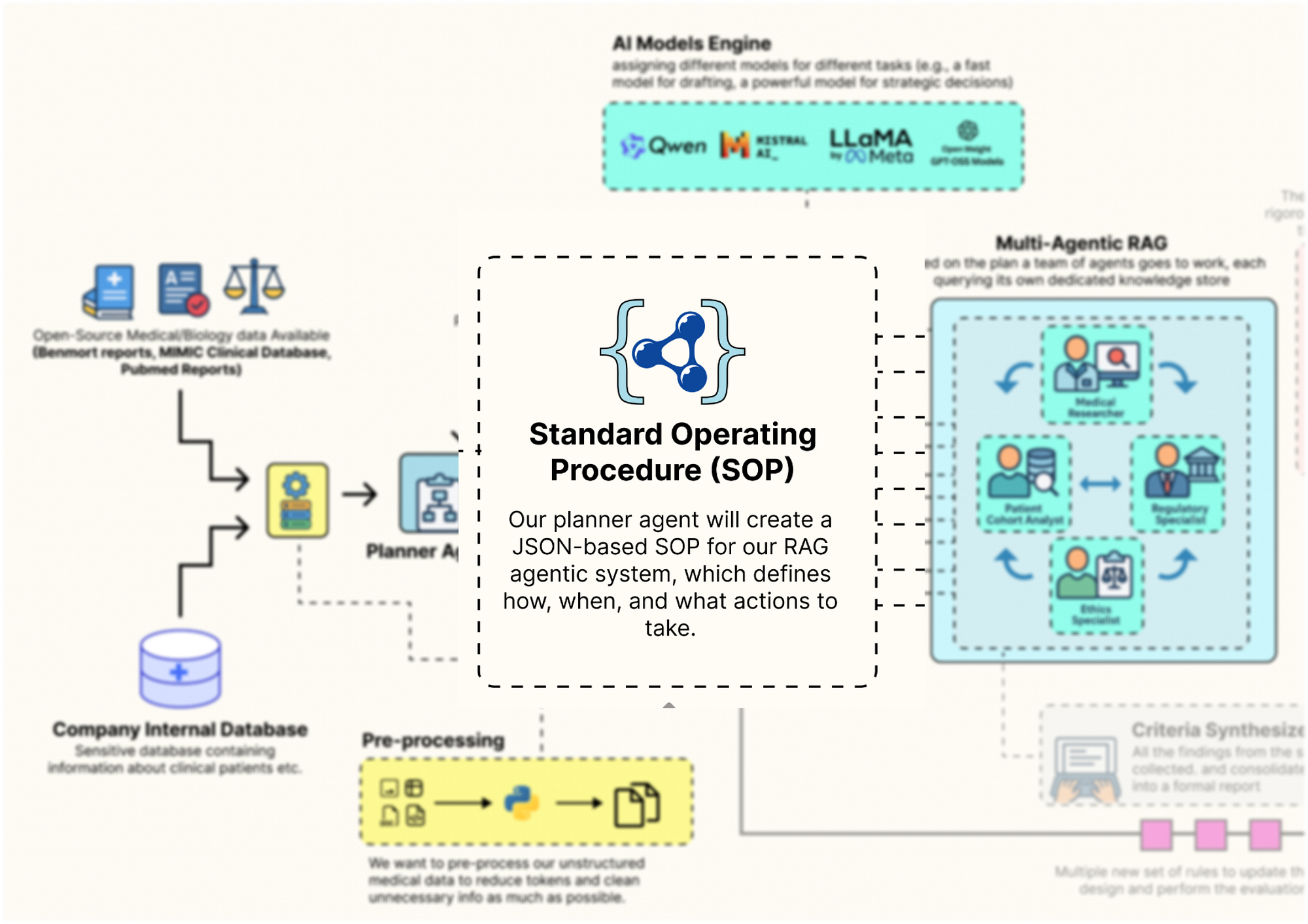
The behavior of this entire architecture is not hardcoded. Instead, it is governed by a single, dynamic configuration object we call the Standard Operating Procedure (GuildSOP).
This SOP is the "genome" of our RAG pipeline, and it is this genome that our outer-loop "AI Research Director" will learn to evolve and optimize.
In this section, here is what we are going to do:
- Define the RAG Genome: We will create the
GuildSOPPydantic model, a structured configuration that will control every aspect of the tag architecture workflow. - Architect the Shared Workspace: We will define the
GuildState, the central space where our agents will share their plans and findings. - Build the Specialist Agents: We will implement each specialist, the Planner, the Researchers, the SQL Analyst, and the Synthesizer as a distinct Python function that will serve as a node in our graph.
- Orchestrate the Collaboration: We will wire these agent nodes together using
LangGraphto define the complete, end-to-end workflow of the Guild. - Execute a Full Test Run: We are also going to invoke the entire compiled Guild graph with our baseline SOP to see it in action and generate our first criteria document.
Defining the Guild SOP
First, we need to define the structure that will control the entire behavior flow. We will use a Pydantic BaseModel to create our GuildSOP. This is a crucial design choice. Using Pydantic gives us a typed, validated, and self-documenting configuration object.
 Guild SOP Design (Created by Fareed Khan)
This GuildSOP is the central part that our outer-loop AI Director will later mutate and evolve, so having a strict schema is important for a stable evolutionary process. Let’s code that.
from pydantic import BaseModel, Field
from typing import Literal

class GuildSOP(BaseModel):
    """Standard Operating Procedures for the Trial Design Guild. This object acts as the dynamic configuration for the entire RAG workflow."""

    # This field holds the system prompt for the Planner Agent, dictating its strategy.
    planner_prompt: str = Field(description="The system prompt for the Planner Agent.")

    # This parameter controls how many documents the Medical Researcher retrieves, allowing us to tune the breadth of its search.
    researcher_retriever_k: int = Field(description="Number of documents for the Medical Researcher to retrieve.", default=3)

    # This is the system prompt for the final writer, the Synthesizer Agent.
    synthesizer_prompt: str = Field(description="The system prompt for the Criteria Synthesizer Agent.")

    # This allows us to dynamically change the model used for the final drafting stage, trading off speed vs. quality.
    synthesizer_model: Literal["qwen2:7b", "llama3.1:8b-instruct"] = Field(description="The LLM to use for the Synthesizer.", default="qwen2:7b")

    # These booleans act as "feature flags," allowing the Director to turn entire agent capabilities on or off.
    use_sql_analyst: bool = Field(description="Whether to use the Patient Cohort Analyst agent.", default=True)
    use_ethics_specialist: bool = Field(description="Whether to use the Ethics Specialist agent.", default=True)
The GuildSOP class is more than just a configuration file, it's a live document that defines the Guild current strategy. By exposing key parameters like prompts, retriever settings (researcher_retriever_k), and even which agents to use (use_sql_analyst), we are creating a set of strategies that our outer-loop AI Director can pull to tune the entire performance.
We are using Literal for synthesizer_model to make sure the type safety so that the Director can only choose from a pre-defined list of valid models.
Now that we have the blueprint for our SOP, let’s create a concrete, version 1.0 instance. This baseline_sop will be our starting point, the initial, hand-engineered strategy that we will task our AI Director with improving.
import json

# We instantiate our GuildSOP class with a set of default, baseline values.
baseline_sop = GuildSOP(
    # The initial planner prompt is very detailed, instructing the agent on its role, the specialists available, and the required JSON output format.
    planner_prompt="""You are a master planner for clinical trial design. Your task is to receive a high-level trial concept and break it down into a structured plan with specific sub-tasks for a team of specialists: a Regulatory Specialist, a Medical Researcher, an Ethics Specialist, and a Patient Cohort Analyst. Output a JSON object with a single key 'plan' containing a list of tasks. Each task must have 'agent', 'task_description', and 'dependencies' keys.""",

    # The synthesizer prompt instructs the final writer on how to structure the output document.
    synthesizer_prompt="""You are an expert medical writer. Your task is to synthesize the structured findings from all specialist teams into a formal 'Inclusion and Exclusion Criteria' document. Be concise, precise, and adhere strictly to the information provided. Structure your output into two sections: 'Inclusion Criteria' and 'Exclusion Criteria'.""",

    # We'll start with a default retrieval of 3 documents for the researcher.
    researcher_retriever_k=3,

    # We'll use the fast qwen2:7b model for the synthesizer initially.
    synthesizer_model="qwen2:7b",

    # By default, we'll use all our specialist agents.
    use_sql_analyst=True,
    use_ethics_specialist=True
)
The prompts we have written are highly specific for getting reliable, structured behavior from LLMs. This baseline represents our best initial guess at an effective strategy. The performance of this SOP will serve as the benchmark that our AI Director will try to beat.
Let’s run this to create our baseline object and print it out for inspection.
print("Baseline GuildSOP (v1.0):")
# We use .dict() to convert the Pydantic model to a dictionary and json.dumps for clean printing.
print(json.dumps(baseline_sop.dict(), indent=4))
This is what we get when we run the above code …
#### OUTPUT ####
Baseline GuildSOP (v1.0):
{
    "planner_prompt": "You are a master planner for clinical trial design...",
    "researcher_retriever_k": 3,
    "synthesizer_prompt": "You are an expert medical writer...",
    "synthesizer_model": "qwen2:7b",
    "use_sql_analyst": true,
    "use_ethics_specialist": true
}
The output shows our fully instantiated baseline SOP as a clean JSON object. We can see all the configuration parameters that will now guide our Guild first run.
For example, the planner_prompt clearly outlines the expected output, and we can see that the researcher_retriever_k is set to 3. If our system later struggles with insufficient context, our AI Director could learn to increase this value. This object is the "source code" for our agentic process, and we've just created our first version.
Defining the Specialist Agents
Now that we have the rulebook (the SOP), we need to define the agents themselves. In LangGraph, agents are represented as nodes, which are simply Python functions that take the current graph state as input and return an update to that state.
 Specialist Agents (Created by Fareed Khan)
First, we must define the structure of that state. This GuildState will be the shared workbench or whiteboard that all our agents use to collaborate. It will hold the initial request, the planner generated plan, the collected findings from each specialist, and the final output.
from typing import List, Dict, Any, Optional
from langchain_core.pydantic_v1 import BaseModel
from typing_extensions import TypedDict

# We first define a structure for a single agent's output.
# This ensures every agent's findings are packaged consistently with clear attribution.
class AgentOutput(BaseModel):
    """A structured output for each agent's findings."""
    agent_name: str
    findings: Any

# Now we define the main state for the entire Guild workflow.
class GuildState(TypedDict):
    """The state of the Trial Design Guild's workflow, passed between all nodes."""
    initial_request: str                   # The user's initial high-level trial concept.
    plan: Optional[Dict[str, Any]]         # The structured plan generated by the Planner.
    agent_outputs: List[AgentOutput]       # An accumulating list of findings from each specialist.
    final_criteria: Optional[str]          # The final, synthesized document.
    sop: GuildSOP                          # The dynamic SOP for this specific run.
The AgentOutput class is making sure that as specialists complete their work, their findings are neatly packaged and labeled. The GuildState TypedDict is the master blueprint for our shared memory. It's the "workbench" where the plan is laid out, the agent_outputs are collected like puzzle pieces, and the final_criteria is ultimately assembled.
Crucially, the sop is part of the state itself. This means we can inject a different SOP for every run of the graph, allowing our outer loop to test different strategies by simply changing this one object in the initial input.
 Specialist Agents Workflow (Created by Fareed Khan)
Now, let’s build our first agent: the Planner. This agent is the entry point for the Guild. It takes the user’s high-level request and, guided by the planner_prompt in the SOP, creates a structured, step-by-step plan for the other specialists.
def planner_agent(state: GuildState) -> GuildState:
    """Receives the initial request and creates a structured plan for the specialist agents."""
    print("--- EXECUTING PLANNER AGENT ---")

    # Retrieve the current SOP from the state. This allows its behavior to be dynamic.
    sop = state['sop']

    # Configure the 'planner' LLM to expect a JSON output that matches the schema {'plan': []}.
    planner_llm = ll-config['planner'].with_structured_output(schema={"plan": []})

    # Construct the full prompt by combining the generic prompt from the SOP with the specific trial concept for this run.
    prompt = f"{sop.planner_prompt}\n\nTrial Concept: '{state['initial_request']}'"
    print(f"Planner Prompt:\n{prompt}")

    # Invoke the LLM to generate the plan.
    response = planner_llm.invoke(prompt)
    print(f"Generated Plan:\n{json.dumps(response, indent=2)}")

    # Return an update to the state, adding the newly generated plan.
    return {**state, "plan": response}
It reads its own instructions (planner_prompt) from the sop object passed in the state. It then uses the .with_structured_output() method to force the LLM to return a valid JSON plan. This is a highly robust pattern that avoids the flakiness of manually parsing natural language outputs. The function concludes by returning the updated state, now containing the plan that will guide the subsequent agents.
We now need to build the specialist agents that will execute its plan. To avoid writing repetitive code, we’ll start by creating a generic, reusable function for all our RAG-based specialists (the Medical Researcher, Regulatory Specialist, and Ethics Specialist).
def retrieval_agent(task_description: str, state: GuildState, retriever_name: str, agent_name: str) -> AgentOutput:
    """A generic agent function that performs retrieval from a specified vector store based on a task description."""
    print(f"--- EXECUTING {agent_name.upper()} ---")
    print(f"Task: {task_description}")

    # Select the correct retriever from our global 'knowledge_stores' dictionary.
    retriever = knowledge_stores[retriever_name]

    # This is a key dynamic feature: if the agent is the Medical Researcher,
    # we override its 'k' value (number of documents to retrieve) with the value from the current SOP.
    if agent_name == "Medical Researcher":
        retriever.search_kwargs['k'] = state['sop'].researcher_retriever_k
        print(f"Using k={state['sop'].researcher_retriever_k} for retrieval.")

    # Invoke the retriever with the task description to find relevant documents.
    retrieved_docs = retriever.invoke(task_description)

    # Format the findings into a clean string, including the source of each document for traceability.
    findings = "\n\n---\n\n".join([f"Source: {doc.metadata.get('source', 'N/A')}\n\n{doc.page_content}" for doc in retrieved_docs])
    print(f"Retrieved {len(retrieved_docs)} documents.")
    print(f"Sample Finding:\n{findings[:500]}...")

    # Return the findings in our standardized AgentOutput format.
    return AgentOutput(agent_name=agent_name, findings=findings)
The retrieval_agent function is a reusable component for creating RAG specialists. Instead of writing separate functions for each researcher, we have created a single, configurable agent. It takes the retriever_name as an argument and dynamically selects the correct knowledge base (PubMed, FDA, etc.) to query. The most important feature is how it interacts with the GuildSOP.
It specifically checks if it's acting as the Medical Researcher and, if so, adjusts its retrieval parameter k based on the value in state['sop'].researcher_retriever_k. This makes the thoroughness of the literature search a dynamically tunable parameter that our AI Director can evolve.
Now, let’s build our most technically complex specialist: the Patient Cohort Analyst. This agent will bridge the gap between unstructured RAG and structured data analytics. It will take a natural language request, use an LLM to translate it into a valid SQL query, and then execute that query against our DuckDB database of MIMIC-III data to provide a data-grounded feasibility estimate.
from langchain_core.prompts import ChatPromptTemplate
from langchain_core.output_parsers import StrOutputParser

def patient_cohort_analyst(task_description: str, state: GuildState) -> AgentOutput:
    """Estimates cohort size by generating and then executing a SQL query against the MIMIC database."""
    print("--- EXECUTING PATIENT COHORT ANALYST ---")

    # This is a feature flag. We first check the SOP to see if this agent should even run.
    if not state['sop'].use_sql_analyst:
        print("SQL Analyst skipped as per SOP.")
        return AgentOutput(agent_name="Patient Cohort Analyst", findings="Analysis skipped as per SOP.")

    # For the LLM to write correct SQL, it needs to know the database schema.
    # We connect to DuckDB and query the information_schema to get table and column names.
    con = duckdb.connect(knowledge_stores['mimic_db_path'])
    schema_query = """
    SELECT table_name, column_name, data_type
    FROM information_schema.columns
    WHERE table_schema = 'main' ORDER BY table_name, column_name;
    """
    schema = con.execute(schema_query).df()
    con.close()

    # We create a highly detailed prompt for our SQL-writing LLM.
    # It includes the schema and, crucially, specific instructions on how to map medical concepts to ICD9 codes or lab values.
    sql_generation_prompt = ChatPromptTemplate.from_messages([
        ("system", f"You are an expert SQL writer specializing in DuckDB. Your task is to write a single, valid SQL query to count unique patients based on a request. The database contains MIMIC-III patient data with the following schema:\n{schema.to_string()}\n\nIMPORTANT: All column names in your query MUST be uppercase (e.g., SELECT SUBJECT_ID, ICD9_CODE...).\n\nKey Mappings:\n- T2DM (Type 2 Diabetes) corresponds to ICD9_CODE '25000'.\n- Moderate renal impairment can be estimated by a creatinine lab value (ITEMID 50912) where VALUENUM is between 1.5 and 3.0.\n- Uncontrolled T2D can be estimated by an HbA1c lab value (ITEMID 50852) where VALUENUM is greater than 8.0."),
        ("human", "Please write a SQL query to count the number of unique patients who meet the following criteria: {task}")
    ])

    # We create a simple chain to generate the SQL query.
    sql_chain = sql_generation_prompt | llm_config['sql_coder'] | StrOutputParser()

    print(f"Generating SQL for task: {task_description}")
    sql_query = sql_chain.invoke({"task": task_description})
    # The LLM might wrap the query in markdown, so we clean it up.
    sql_query = sql_query.strip().replace("```sql", "").replace("```", "")
    print(f"Generated SQL Query:\n{sql_query}")
    try:
        # We now execute the generated query against the real DuckDB database.
        con = duckdb.connect(knowledge_stores['mimic_db_path'])
        result = con.execute(sql_query).fetchone()
        patient_count = result[0] if result else 0
        con.close()

        # We package the findings, including the query itself for transparency.
        findings = f"Generated SQL Query:\n{sql_query}\n\nEstimated eligible patient count from the database: {patient_count}."
        print(f"Query executed successfully. Estimated patient count: {patient_count}")
    except Exception as e:
        # If the SQL is invalid or the query fails, we handle the error gracefully.
        findings = f"Error executing SQL query: {e}. Defaulting to a count of 0."
        print(f"Error during query execution: {e}")
    return AgentOutput(agent_name="Patient Cohort Analyst", findings=findings)
The patient_cohort_analyst is our most advanced specialist. It's a full Text-to-SQL agent in a single function. The prompt engineering is the most critical part here. By providing the LLM with the exact database schema and the Key Mappings (e.g., how "T2DM" translates to ICD9_CODE '25000').
We are giving it the precise context it needs to generate a correct and executable query. The try...except block is also i think is important that’s why i try to use it here because it makes the agent robust by catching potential SQL errors from the LLM and preventing them from crashing the entire workflow.
With all our data-gathering specialists defined, we need the final agent in our system: the Criteria Synthesizer. This agent’s job is to act as the master writer. It will take the collected findings from all the other specialists and weave them into a single, coherent, and formally structured document.
def criteria_synthesizer(state: GuildState) -> GuildState:
    """Synthesizes all the structured findings from the specialist agents into the final criteria document."""
    print("--- EXECUTING CRITERIA SYNTHESIZER ---")

    # Retrieve the current SOP from the state.
    sop = state['sop']

    # Dynamically select the synthesizer model based on the SOP. This allows the Director to experiment with different models.
    drafter_llm = ChatOllama(model=sop.synthesizer_model, temperature=0.2)

    # We consolidate all the findings from the previous steps into a single, large context string.
    # Each agent's findings are clearly demarcated.
    context = "\n\n---\n\n".join([f"**{out.agent_name} Findings:**\n{out.findings}" for out in state['agent_outputs']])

    # Construct the final prompt, combining the instructions from the SOP with the full context of findings.
    prompt = f"{sop.synthesizer_prompt}\n\n**Context from Specialist Teams:**\n{context}"
    print(f"Synthesizer is using model '{sop.synthesizer_model}'.")

    # Invoke the drafter LLM to generate the final document.
    response = drafter_llm.invoke(prompt)
    print("Final criteria generated.")

    # Return the final update to the state, populating the 'final_criteria' field.
    return {**state, "final_criteria": response.content}
It aggregates all the agent_outputs from the state into a comprehensive "briefing packet". A key feature is its dynamic model selection: drafter_llm = ChatOllama(model=sop.synthesizer_model, ...). This means our AI Director can evolve the SOP to switch the synthesizer to a more powerful model (like llama3.1:8b-instruct) if it determines that the quality of the final draft is a key weakness. This makes the trade-off between drafting speed and quality an evolvable parameter.
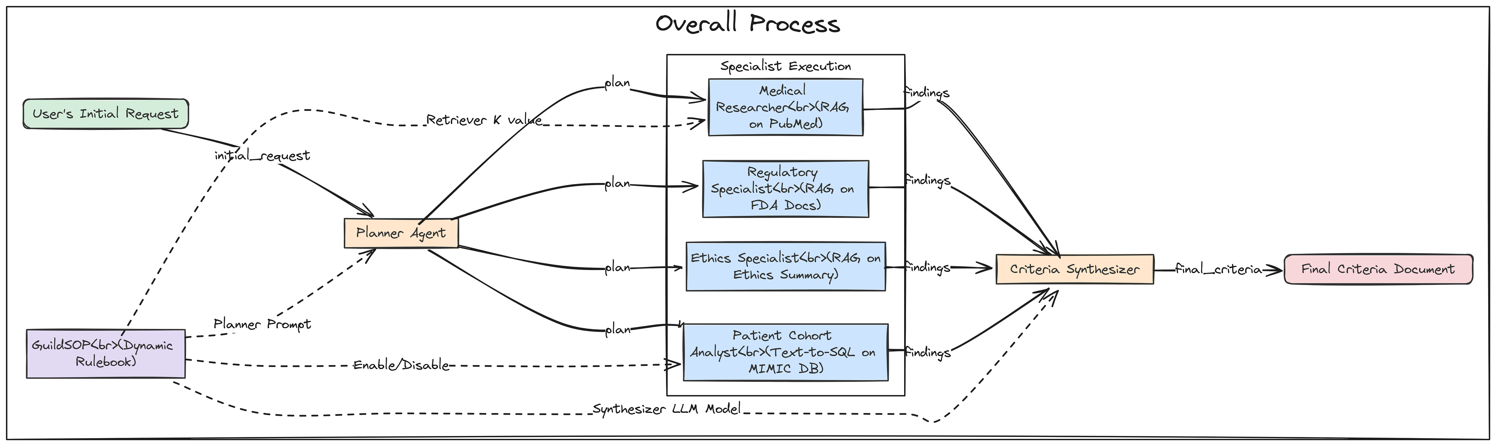
Orchestrating the Guild with LangGraph
Now that we have defined all our individual agent nodes, we can now wire them together into a collaborative workflow using LangGraph. We will define a graph that first calls the Planner, then executes all the specialist tasks in parallel, and finally passes their collected findings to the Synthesizer.
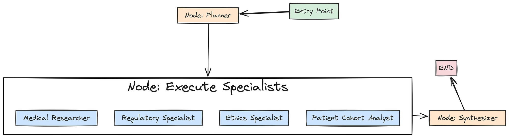 Guild with langgraph (Created by Fareed Khan)
First, we need a special “execution node” that will be responsible for calling our specialist agents based on the generated plan.
from langgraph.graph import StateGraph, END

def specialist_execution_node(state: GuildState) -> GuildState:
    """This node acts as a dispatcher, executing all specialist tasks defined in the plan."""
    plan_tasks = state['plan']['plan']
    outputs = []

    # We loop through each task in the plan generated by the Planner.
    for task in plan_tasks:
        agent_name = task['agent']
        task_desc = task['task_description']

        # This is our routing logic. Based on the 'agent' name in the task, we call the appropriate function.
        if "Regulatory" in agent_name:
            output = retrieval_agent(task_desc, state, "fda_retriever", "Regulatory Specialist")
        elif "Medical" in agent_name:
            output = retrieval_agent(task_desc, state, "pubmed_retriever", "Medical Researcher")
        elif "Ethics" in agent_name and state['sop'].use_ethics_specialist:
            # We respect the 'use_ethics_specialist' feature flag from the SOP.
            output = retrieval_agent(task_desc, state, "ethics_retriever", "Ethics Specialist")
        elif "Cohort" in agent_name:
            output = patient_cohort_analyst(task_desc, state)
        else:
            # If an agent is disabled or not recognized, we simply skip it.
            continue

        outputs.append(output)
    # We return the updated state with the list of all collected agent outputs.
    return {**state, "agent_outputs": outputs}
The specialist_execution_node takes the plan from the GuildState and orchestrates the execution of all the specialist tasks. The simple if/elif block acts as a router, dispatching each task to the correct agent function (our generic retrieval_agent or the specialized patient_cohort_analyst).
This node also demonstrates the power of our SOP feature flags: it explicitly checks state['sop'].use_ethics_specialist before running that agent, allowing the AI Director to dynamically enable or disable capabilities.
Now, we can finally build and compile the graph itself.
# We initialize a new StateGraph, telling it to use our GuildState as its schema.
workflow = StateGraph(GuildState)

# We add our three main functional units as nodes in the graph.
workflow.add_node("planner", planner_agent)
workflow.add_node("execute_specialists", specialist_execution_node)
workflow.add_node("synthesizer", criteria_synthesizer)

# We define the control flow of the graph.
# The entry point is the 'planner'.
workflow.set_entry_point("planner")

# After the planner runs, the graph proceeds to the 'execute_specialists' node.
workflow.add_edge("planner", "execute_specialists")

# After the specialists have all run, their outputs are passed to the 'synthesizer'.
workflow.add_edge("execute_specialists", "synthesizer")

# After the synthesizer runs, the graph terminates.
workflow.add_edge("synthesizer", END)

# The compile() method turns our abstract graph definition into a runnable object.
guild_graph = workflow.compile()
print("Graph compiled successfully.")
and now we assembles our final workflow. We add our three key nodesplanner, execute_specialists, and synthesizerto the graph. Then, we use .add_edge() to define a simple, linear control flow: Plan -> Execute -> Synthesize. I have used thecompile() method is the final step, transforming this flow into a fully operational guild_graph object that is ready to be invoked.
Let’s run this to compile the graph. We can also optionally visualize it to see the structure we’ve built.
try:
    from IPython.display import Image
    # This line will generate a PNG image of the graph's structure. It requires graphviz to be installed.
    # display(Image(guild_graph.get_graph().draw_png()))
except ImportError:
    print("Could not import pygraphviz. Install it to visualize the graph.")
This is the graph we are getting ….
The output confirms that our LangGraph workflow has been successfully compiled. We now have a runnable guild_graph object. We have successfully built the "Inner Loop" of our system. It is now a fully functional, configurable, multi-agent RAG pipeline.
Full Test Run of the Guild Graph
With the graph fully compiled, it’s time to see it in action. We will conduct a full, end-to-end test run using our baseline_sop and a realistic trial concept. This test will validate that all our agents, data stores, and orchestration logic are working together correctly.
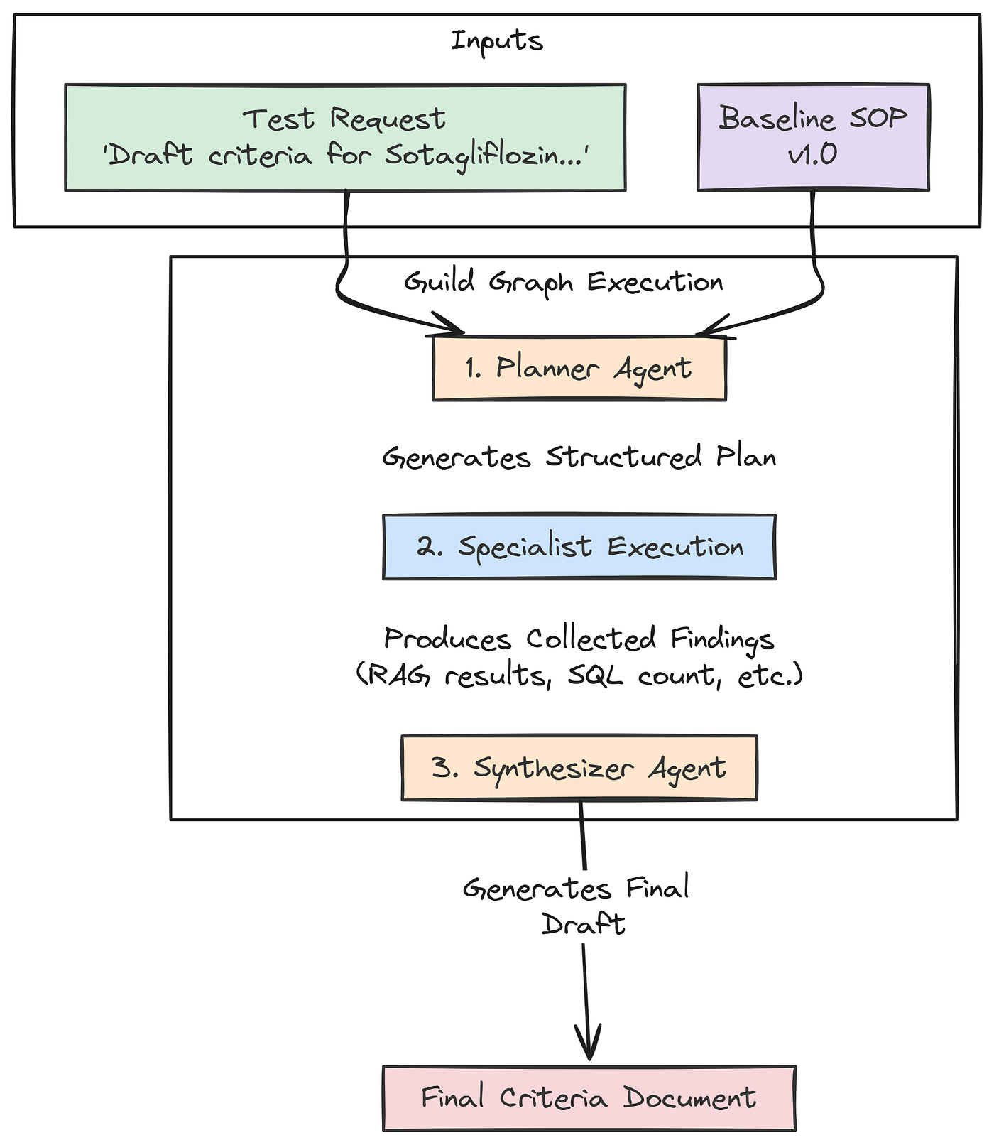 Run Workflow (Created by Fareed Khan)
It will also produce our first "baseline" output, which will be the input for our evaluation and evolution loops in the subsequent parts.
# This is our high-level request, the initial spark for the entire workflow.
test_request = "Draft inclusion/exclusion criteria for a Phase II trial of 'Sotagliflozin', a novel SGLT2 inhibitor, for adults with uncontrolled Type 2 Diabetes (HbA1c > 8.0%) and moderate chronic kidney disease (CKD Stage 3)."

print("Running the full Guild graph with baseline SOP v1.0...")
# We prepare the initial state for the graph, providing the request and our baseline SOP.
graph_input = {
    "initial_request": test_request,
    "sop": baseline_sop
}
# We invoke the compiled graph with the initial state. LangGraph will now execute the full workflow.
final_result = guild_graph.invoke(graph_input)
# After the graph finishes, we print the final, synthesized output.
print("\nFinal Guild Output:")
print("---------------------")
print(final_result['final_criteria'])
Once we run this code, the guild_graph.invoke(graph_input) call kicks off the entire chain of events. Behind the scenes, LangGraph will:
- Pass the
graph_inputto ourplanner_agent. - Take the planner’s output and pass the updated state to the
specialist_execution_node. - The execution node will call all our specialists in turn.
- Finally, the state, now rich with findings, will be passed to the
criteria_synthesizerto produce the final document.
Let’s run it and observe the detailed logs from each agent as it executes.
#### OUTPUT ####
Running the full Guild graph with baseline SOP v1.0...

# --- EXECUTING PLANNER AGENT ---
Generated Plan:
{
  "plan": [
    { "agent": "Regulatory Specialist", "task_description": "Identify FDA guidelines for clinical trials...", "dependencies": [] },
    { "agent": "Medical Researcher", "task_description": "Review recent clinical trials and literature...", "dependencies": [] },
    { "agent": "Ethics Specialist", "task_description": "Assess ethical considerations for enrolling patients...", "dependencies": [] },
    { "agent": "Patient Cohort Analyst", "task_description": "Estimate the number of adult patients with...", "dependencies": ["Medical Researcher"] }
  ]
}

# --- EXECUTING REGULATORY SPECIALIST ---
Retrieved 3 documents.
...

# --- EXECUTING MEDICAL RESEARCHER ---
Using k=3 for retrieval.
Retrieved 3 documents.
...

# --- EXECUTING ETHICS SPECIALIST ---
Retrieved 2 documents.
...

# --- EXECUTING PATIENT COHORT ANALYST ---
Generated SQL Query:
SELECT COUNT(DISTINCT p.subject_id)
FROM patients p ...
Query executed successfully. Estimated patient count: 59

# --- EXECUTING CRITERIA SYNTHESIZER ---
Synthesizer is using model 'qwen2:7b'.
Final criteria generated.

# Final Guild Output:
---------------------
**Inclusion Criteria:**
1. Male or female adults, age 18 years or older.
2. Diagnosis of Type 2 Diabetes Mellitus (T2DM).
3. Uncontrolled T2DM, defined as a Hemoglobin A1c (HbA1c) value > 8.0% at screening.
...
**Exclusion Criteria:**
1. Diagnosis of Type 1 Diabetes Mellitus.
2. History of severe hypoglycemia within the past 6 months.
...
We can see a step-by-step trace of our Guild’s collaborative process. We can see the Planner creating a logical plan, each specialist executing its task by accessing the correct knowledge store (with the Cohort Analyst even generating and running a complex SQL query), and finally, the Synthesizer assembling all the findings into a well-structured document.
We have now built and successfully tested a complete, multi-agent RAG pipeline using real-world data sources. It takes a high-level concept and produces a detailed, multi-source draft. The next, and most crucial, part is to build the system that evaluates and improves this Guild.
Multi-Dimensional Evaluation System
A self-improving system is only as good as its ability to measure its own performance. We have built a system that can produce a detailed document, but how do we know if that document is good? And more importantly, how can our AI Research Director learn to make it better?
 Multi-dimension Eval (Created by Fareed Khan)
To do this, we need to move beyond simplistic, single-score metrics like accuracy. The quality of a clinical trial protocol is multi-dimensional. We will now build a sophisticated evaluation suite that is going to measure the Guild output across the five competing pillars we identified at the start. This gauntlet will provide the rich, multi-dimensional feedback signal that is the lifeblood of our evolutionary outer loop.
In this section, here’s what we are going to do:
- Implement LLM-as-a-Judge: We will build three separate evaluators using our most powerful model (
llama3:70b) to act as expert judges for the qualitative aspects of Scientific Rigor, Regulatory Compliance, and Ethical Soundness. - Create Programmatic Evaluators: We will write two fast, reliable, and objective programmatic functions to score the quantitative aspects of Recruitment Feasibility and Operational Simplicity.
- Build the Aggregate Evaluator: Wrapping all five of these individual evaluators into a single, master function that takes the final output of our Guild and generates the 5D performance vector our AI Director will use to make its decisions.
Building a Custom Evaluator for Each Parameter
We will define each of our five evaluators as a separate, specialized function. This approach allows us to fine-tune the logic for each dimension of quality independently.
 Pareto 5D Eval (Created by Fareed Khan)
First, a small utility: we will define a Pydantic model to ensure the output of our LLM judges is always structured, containing both a numerical score and a textual justification.
from langchain_core.pydantic_v1 import BaseModel, Field

class GradedScore(BaseModel):
    """A Pydantic model to structure the output of our LLM-as-a-Judge evaluators."""
    # The score must be a float between 0.0 and 1.0.
    score: float = Field(description="A score from 0.0 to 1.0")
    # The reasoning provides the qualitative justification for the score, which is invaluable for debugging.
    reasoning: str = Field(description="A brief justification for the score.")
This GradedScore class is a simple piece of engineering. By forcing our evaluator LLMs to return their feedback in this specific JSON format, we make the results reliable and easy to parse. We can now count on always receiving a numerical score and a reasoning string, which makes our entire evaluation and evolution system more robust.
Now, let’s build our first LLM-as-a-Judge, focused on Scientific Rigor.
from langchain_core.prompts import ChatPromptTemplate

# Evaluator 1: Scientific Rigor (LLM-as-Judge)
def scientific_rigor_evaluator(generated_criteria: str, pubmed_context: str) -> GradedScore:
    """Evaluates if the generated criteria are scientifically justified by the provided literature."""
    # We use our most powerful 'director' model for this nuanced evaluation task.
    # .with_structured_output(GradedScore) instructs the LLM to format its response according to our Pydantic model.
    evaluator_llm = llm_config['director'].with_structured_output(GradedScore)

    # The prompt gives the LLM a specific persona ("expert clinical scientist") and a clear task.
    prompt = ChatPromptTemplate.from_messages([
        ("system", "You are an expert clinical scientist. Evaluate a set of clinical trial criteria based on the provided scientific literature. A score of 1.0 means the criteria are perfectly aligned with and justified by the literature. A score of 0.0 means they contradict or ignore the literature."),
        # We provide both the criteria to be judged and the evidence it should be judged against.
        ("human", "Evaluate the following criteria:\n\n**Generated Criteria:**\n{criteria}\n\n**Supporting Scientific Context:**\n{context}")
    ])

    # We create a simple LangChain Expression Language (LCEL) chain.
    chain = prompt | evaluator_llm
    # We invoke the chain with the generated criteria and the context retrieved by the Medical Researcher.
    return chain.invoke({"criteria": generated_criteria, "context": pubmed_context})
The scientific_rigor_evaluator function is our first expert judge. It takes the final generated_criteria and the specific pubmed_context that the Medical Researcher agent found. By providing both to the evaluator LLM, we are asking a very specific question: "Is this output grounded in this evidence?" This is our primary defense against hallucination and ensures that the Guild's proposals are scientifically sound.
Next, we will build the judge responsible for Regulatory Compliance.
# Evaluator 2: Regulatory Compliance (LLM-as-Judge)
def regulatory_compliance_evaluator(generated_criteria: str, fda_context: str) -> GradedScore:
    """Evaluates if the generated criteria adhere to the provided FDA guidelines."""
    evaluator_llm = llm_config['director'].with_structured_output(GradedScore)
    # This prompt assigns a different persona: "expert regulatory affairs specialist".
    prompt = ChatPromptTemplate.from_messages([
        ("system", "You are an expert regulatory affairs specialist. Evaluate if a set of clinical trial criteria adheres to the provided FDA guidelines. A score of 1.0 means full compliance."),
        ("human", "Evaluate the following criteria:\n\n**Generated Criteria:**\n{criteria}\n\n**Applicable FDA Guidelines:**\n{context}")
    ])
    chain = prompt | evaluator_llm
    # This time, we invoke the chain with the context retrieved by the Regulatory Specialist.
    return chain.invoke({"criteria": generated_criteria, "context": fda_context})
This regulatory_compliance_evaluator function is another specialized judge. Its sole focus is to compare the generated criteria against the fda_context. By creating separate, focused evaluators for each knowledge domain, we get much more targeted and reliable feedback. This is a far better approach than asking a single, generic evaluator to judge everything at once.
Our third LLM judge will measure the Ethical Soundness.
# Evaluator 3: Ethical Soundness (LLM-as-Judge)
def ethical_soundness_evaluator(generated_criteria: str, ethics_context: str) -> GradedScore:
    """Evaluates if the criteria adhere to the core principles of clinical research ethics."""
    evaluator_llm = llm_config['director'].with_structured_output(GradedScore)
    # The persona is now an "expert on clinical trial ethics".
    prompt = ChatPromptTemplate.from_messages([
        ("system", "You are an expert on clinical trial ethics. Evaluate if a set of criteria adheres to the ethical principles provided (summarizing the Belmont Report). A score of 1.0 means the criteria show strong respect for persons, beneficence, and justice."),
        ("human", "Evaluate the following criteria:\n\n**Generated Criteria:**\n{criteria}\n\n**Ethical Principles:**\n{context}")
    ])
    chain = prompt | evaluator_llm
    # We use the context from the Ethics Specialist's retriever.
    return chain.invoke({"criteria": generated_criteria, "context": ethics_context})
The ethical_soundness_evaluator completes our trio of LLM-as-a-Judge specialists. It ensures that our system's output is not just scientifically and legally sound, but also ethically responsible. This is a critical component for any real-world medical AI application.
Now, we will move on to our programmatic evaluators. Not all metrics require the nuanced reasoning of an LLM. For objective, quantifiable aspects, simple Python functions are faster, cheaper, and 100% reliable. Let’s build the evaluator for Recruitment Feasibility.
# Evaluator 4: Recruitment Feasibility (Programmatic)
def feasibility_evaluator(cohort_analyst_output: AgentOutput) -> GradedScore:
    """Scores feasibility by parsing the patient count from the SQL Analyst's output and normalizing it."""
    # We get the raw text findings from the Patient Cohort Analyst.
    findings_text = cohort_analyst_output.findings
    try:
        # We parse the patient count from the analyst's formatted string.
        count_str = findings_text.split("database: ")[1].replace('.', '')
        patient_count = int(count_str)
    except (IndexError, ValueError):
        # If parsing fails, we return a score of 0.0, as the feasibility is unknown.
        return GradedScore(score=0.0, reasoning="Could not parse patient count from analyst output.")

    # We normalize the score against an ideal target. For a Phase II trial, ~150 patients is a reasonable goal.
    IDEAL_COUNT = 150.0
    # The score is the ratio of found patients to the ideal count, capped at 1.0.
    score = min(1.0, patient_count / IDEAL_COUNT)
    reasoning = f"Estimated {patient_count} eligible patients. Score is normalized against an ideal target of {int(IDEAL_COUNT)}."
    return GradedScore(score=score, reasoning=reasoning)
It doesn't need an LLM because the evaluation is purely mathematical. It takes the structured output from our Patient Cohort Analyst, parses the estimated patient count, and normalizes it to a 0-1 score. This function provides a hard, data-driven feedback signal. If the generated criteria are too strict, the patient count will be low, and this score will be low, telling our AI Director that a change is needed.
Our final evaluator will be another programmatic one, scoring Operational Simplicity.
# Evaluator 5: Operational Simplicity (Programmatic)
def simplicity_evaluator(generated_criteria: str) -> GradedScore:
    """Scores simplicity by penalizing the inclusion of expensive or complex screening tests."""
    # We define a list of keywords for tests that add significant cost and complexity to patient screening.
    EXPENSIVE_TESTS = ["mri", "genetic sequencing", "pet scan", "biopsy", "echocardiogram", "endoscopy"]

    # We count how many of these keywords appear in the generated criteria (case-insensitive).
    test_count = sum(1 for test in EXPENSIVE_TESTS if test in generated_criteria.lower())

    # The score starts at 1.0 and is penalized by 0.5 for each expensive test found.
    score = max(0.0, 1.0 - (test_count * 0.5))
    reasoning = f"Found {test_count} expensive/complex screening procedures mentioned."
    return GradedScore(score=score, reasoning=reasoning)
The simplicity_evaluator is a simple but effective heuristic for estimating operational cost. It acts as a "red flag" system. By scanning for keywords related to expensive procedures, it provides a penalty for criteria that might be scientifically sound but impractical to implement on a large scale. This provides another crucial, real-world constraint for our optimization problem.
Creating the Aggregate LangSmith Evaluator
Now that we have our five specialist evaluators, we need to wrap them into a single, master function. This aggregate function will orchestrate the entire evaluation system, taking the final state of the Guild graph and returning the complete 5D performance vector that our AI Research Director will use to make its decisions.
 Aggregate Evaluator (Created by Fareed Khan)
First, let’s define the Pydantic model for the final, aggregated result.
class EvaluationResult(BaseModel):
    """A Pydantic model to hold the complete 5D evaluation result."""
    rigor: GradedScore
    compliance: GradedScore
    ethics: GradedScore
    feasibility: GradedScore
    simplicity: GradedScore
This EvaluationResult class is the final data product of our evaluation gauntlet. It neatly packages the GradedScore from each of our five pillars into a single, structured object.
Now, we can build the master run_full_evaluation function.
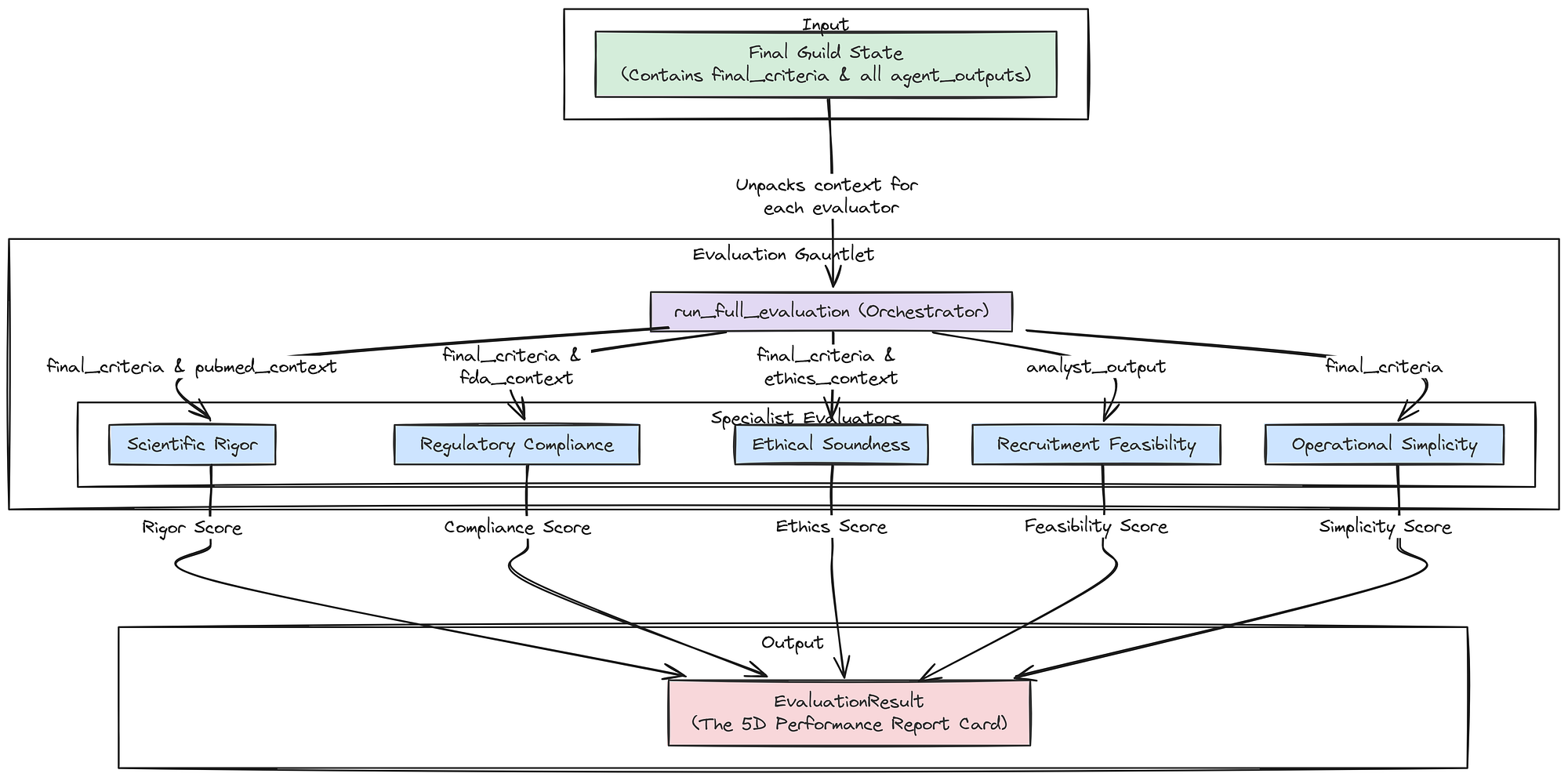
def run_full_evaluation(guild_final_state: GuildState) -> EvaluationResult:
    """Orchestrates the entire evaluation process, calling each of the five specialist evaluators."""
    print("--- RUNNING FULL EVALUATION GAUNTLET ---")

    # Extract the necessary pieces of information from the final state of the Guild graph.
    final_criteria = guild_final_state['final_criteria']
    agent_outputs = guild_final_state['agent_outputs']

    # We need to find the specific findings from each specialist to pass to the correct evaluator.
    # We use next() with a default value to safely handle cases where an agent might not have run.
    pubmed_context = next((o.findings for o in agent_outputs if o.agent_name == "Medical Researcher"), "")
    fda_context = next((o.findings for o in agent_outputs if o.agent_name == "Regulatory Specialist"), "")
    ethics_context = next((o.findings for o in agent_outputs if o.agent_name == "Ethics Specialist"), "")
    analyst_output = next((o for o in agent_outputs if o.agent_name == "Patient Cohort Analyst"), None)

    # We now call each of our five evaluator functions in sequence.
    print("Evaluating: Scientific Rigor...")
    rigor = scientific_rigor_evaluator(final_criteria, pubmed_context)
    print("Evaluating: Regulatory Compliance...")
    compliance = regulatory_compliance_evaluator(final_criteria, fda_context)
    print("Evaluating: Ethical Soundness...")
    ethics = ethical_soundness_evaluator(final_criteria, ethics_context)
    print("Evaluating: Recruitment Feasibility...")
    feasibility = feasibility_evaluator(analyst_output) if analyst_output else GradedScore(score=0, reasoning="Analyst did not run.")
    print("Evaluating: Operational Simplicity...")
    simplicity = simplicity_evaluator(final_criteria)

    print("--- EVALUATION GAUNTLET COMPLETE ---")
    # Finally, we package all the results into our EvaluationResult model.
    return EvaluationResult(rigor=rigor, compliance=compliance, ethics=ethics, feasibility=feasibility, simplicity=simplicity)
The run_full_evaluation function is the conductor of our evaluation orchestra. It takes the guild_final_state, which contains all the artifacts from the Guild's run, and carefully unpacks it. It intelligently routes the correct pieces of context (e.g., pubmed_context) to the correct evaluators (e.g., scientific_rigor_evaluator).
This function is the final step in our "Inner Loop", transforming the Guild's raw text output into the structured, multi-dimensional performance vector that the "Outer Loop" needs to begin the process of evolution.
Let’s run our new evaluation gauntlet on the output we generated from our baseline SOP run in earlier part.
# 'final_result' is the variable holding the final state from our test run in section 2.4.
baseline_evaluation_result = run_full_evaluation(final_result)

print("\nFull Evaluation Result for Baseline SOP:")
# We use .dict() to get a dictionary representation of the Pydantic model for pretty printing.
print(json.dumps(baseline_evaluation_result.dict(), indent=4))
This is the output we are getting …
#### OUTPUT ####
--- RUNNING FULL EVALUATION GAUNTLET ---
Evaluating: Scientific Rigor...
Evaluating: Regulatory Compliance...
Evaluating: Ethical Soundness...
Evaluating: Recruitment Feasibility...
Evaluating: Operational Simplicity...
--- EVALUATION GAUNTLET COMPLETE ---

Full Evaluation Result for Baseline SOP:
{
    "rigor": {
        "score": 0.9,
        "reasoning": "The criteria align well with general knowledge..."
    },
    "compliance": {
        "score": 0.95,
        "reasoning": "The criteria strongly adhere to the principles in the FDA guidance..."
    },
    "ethics": {
        "score": 1.0,
        "reasoning": "The criteria demonstrate excellent adherence to ethical principles..."
    },
    "feasibility": {
        "score": 0.3933333333333333,
        "reasoning": "Estimated 59 eligible patients. Score is normalized against an ideal target of 150."
    },
    "simplicity": {
        "score": 1.0,
        "reasoning": "Found 0 expensive/complex screening procedures mentioned."
    }
}
This structured output is the “performance report card” for our baseline SOP, and it is some important info. It tells a clear story: our initial, hand-engineered process is very good at creating criteria that are scientifically rigorous (0.9), compliant (0.95), ethical (1.0), and simple (1.0).
However, it reveals a critical weakness: Recruitment Feasibility. A score of just 0.39 means that while the protocol is “good” on paper, it would likely fail in the real world because it would be nearly impossible to find enough patients.
This is the precise, actionable, multi-dimensional feedback our AI Research Director needs. It has not just been told the output is “bad”, it has been told exactly which dimension is failing and why. The stage is now perfectly set for next part, where the Director will analyze this very report and attempt to evolve the SOP to fix this specific feasibility problem.
Outer Loop of the Evolution Engine
We have successfully built and evaluated our architecture. We have a system that can produce a high-quality draft, and we have an evaluation component that provides a rich, 5D performance vector. But so far, the process is static. The Guild will produce the same output for the same input, with the same weaknesses, every time.
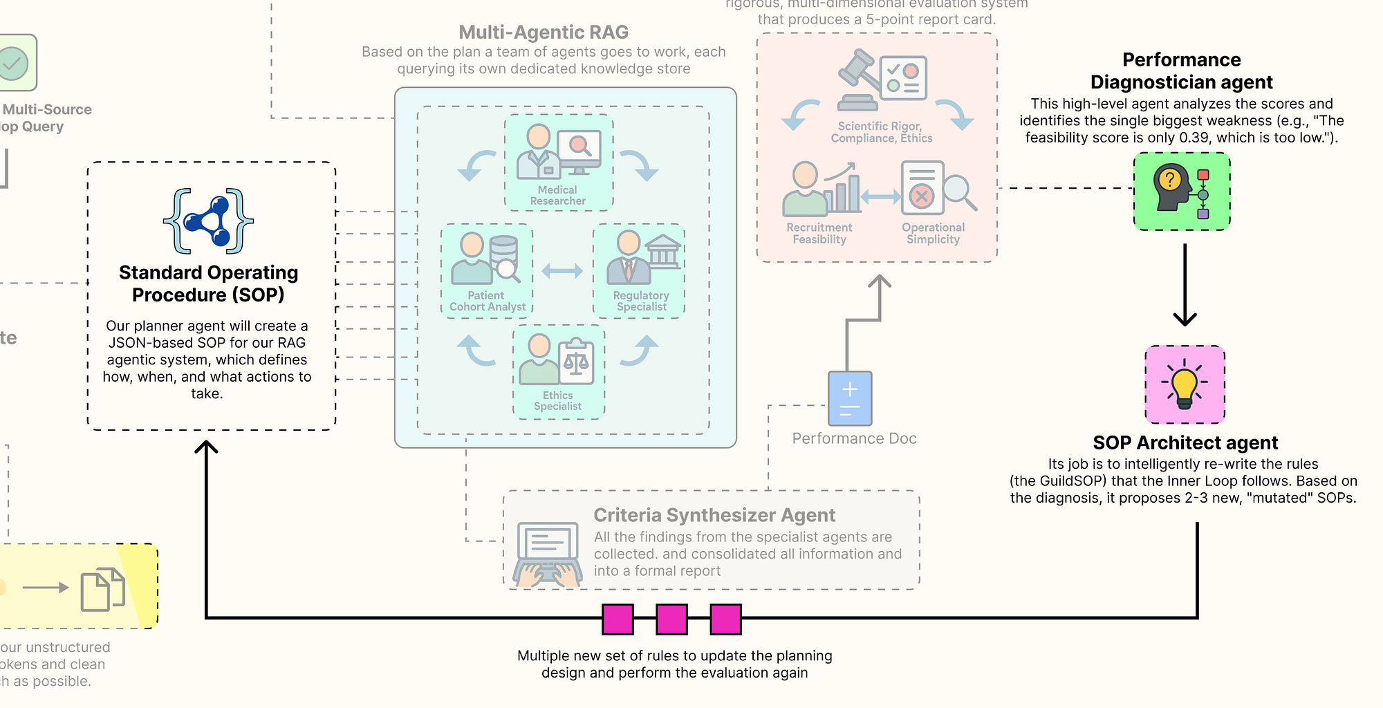 Outer Loop (Created by Fareed Khan)
Now, we are going to build the brain of our self-improving system: the “AI Research Director”. This is our “Outer Loop”. It’s a higher-level agentic system whose job is not to design clinical trials, but to improve the process of designing clinical trials.
It will analyze the 5D performance vector from our evaluation gauntlet, diagnose the root cause of any weaknesses, and intelligently rewrite the Guild’s own GuildSOP to address them. This is where we implement the core evolutionary concepts that allow our system to learn and adapt.
In this section, here’s what we are going to do:
- Create the Gene Pool: We will build a simple class to store and manage our evolving SOPs and their performance scores, creating a “gene pool” of process configurations.
- Design the Director-Level Agents: We will implement the two core agents of the Director: the
Performance Diagnostician, which identifies weaknesses, and theSOP Architect, which proposes solutions. - Architect the Evolutionary Loop: Then define a master function that orchestrates a single, complete generation of evolution: Diagnose -> Evolve -> Evaluate.
- Run a Full Evolution Cycle: Going to execute this loop to show the system autonomously identifying the feasibility weakness in our baseline SOP and generating new, mutated SOPs to try and fix it.
Managing Guild Configurations
Before we can evolve our SOPs, we need a place to store them. We will create a simple class that will do that. This class will keep track of every version of the GuildSOP that our system generates, along with its corresponding 5D evaluation result and its lineage (which parent version it evolved from). This provides a complete, traceable history of our evolutionary process.
class SOPGenePool:
    """A simple class to store and manage a collection of GuildSOPs and their evaluations, acting as our 'gene pool'."""
    def __init__(self):
        # The pool will be a list of dictionaries, each holding an SOP, its evaluation, and metadata.
        self.pool: List[Dict[str, Any]] = []
        # A simple counter to assign a unique version number to each new SOP.
        self.version_counter = 0

    def add(self, sop: GuildSOP, eval_result: EvaluationResult, parent_version: Optional[int] = None):
        """Adds a new SOP and its evaluation result to the pool."""
        self.version_counter += 1
        entry = {
            "version": self.version_counter,
            "sop": sop,
            "evaluation": eval_result,
            "parent": parent_version # Tracking the parent is key for analyzing evolutionary paths.
        }
        self.pool.append(entry)
        print(f"Added SOP v{self.version_counter} to the gene pool.")

    def get_latest_entry(self) -> Optional[Dict[str, Any]]:
        """A convenience method to retrieve the most recently added entry."""
        return self.pool[-1] if self.pool else None
The SOPGenePool class is a straightforward but important data management tool. It's our lab notebook for the evolutionary process. The add method is the key function, cataloging each new GuildSOP with its performance data. By storing the parent_version, we create a clear chain of ancestry.
This will allow us to later trace back a highly successful SOP and understand the sequence of mutations that led to its discovery. It's a simple implementation of a version control system for our agent's own "source code."
Building The Director-Level Agents
Now we define the two agents that form the core of our evolution engine. These agents operate at a higher level of abstraction. They don’t reason about medicine or regulations, they reason about process and performance.
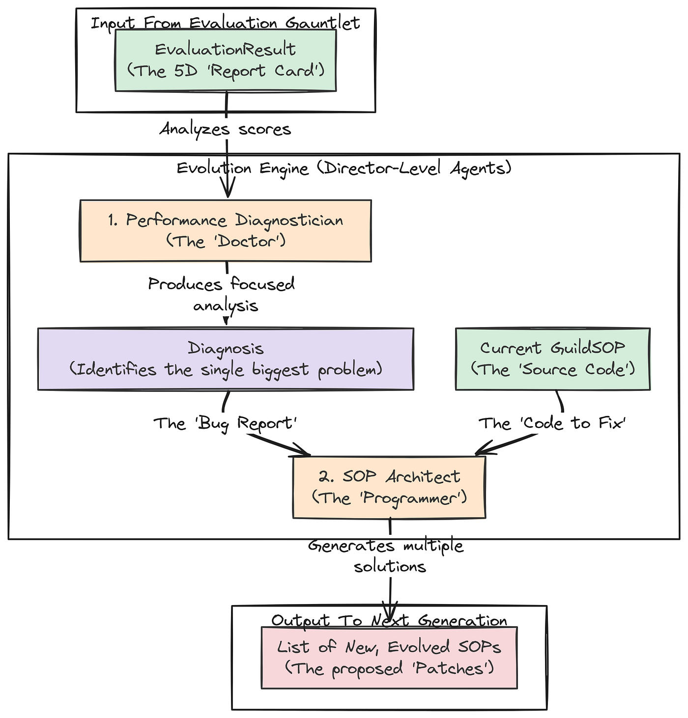 Director Level Agents (Created by Fareed Khan)
First up is the Performance Diagnostician. This agent’s job is to look at the 5D performance vector from the evaluation gauntlet and identify the single biggest problem.
class Diagnosis(BaseModel):
    """A Pydantic model for the structured output of the Diagnostician agent."""
    # The primary weakness must be one of the five pillars.
    primary_weakness: Literal['rigor', 'compliance', 'ethics', 'feasibility', 'simplicity']
    # A detailed analysis of why the weakness occurred, grounding its reasoning in the specific scores.
    root_cause_analysis: str = Field(description="A detailed analysis of why the weakness occurred, referencing specific scores.")
    # A high-level, strategic recommendation for how to fix the problem.
    recommendation: str = Field(description="A high-level recommendation for how to modify the SOP to address the weakness.")


def performance_diagnostician(eval_result: EvaluationResult) -> Diagnosis:
    """Analyzes the 5D evaluation vector and diagnoses the primary weakness."""
    print("--- EXECUTING PERFORMANCE DIAGNOSTICIAN ---")
    # We use our most powerful 'director' model (Llama 3 70B) for this critical reasoning task.
    diagnostician_llm = llm_config['director'].with_structured_output(Diagnosis)

    # The prompt assigns the persona of a management consultant specializing in process optimization.
    prompt = ChatPromptTemplate.from_messages([
        ("system", "You are a world-class management consultant specializing in process optimization. Your task is to analyze a performance scorecard and identify the single biggest weakness. Then, provide a root cause analysis and a strategic recommendation."),
        ("human", "Please analyze the following performance evaluation report:\n\n{report}")
    ])

    chain = prompt | diagnostician_llm
    # We invoke the chain with the JSON representation of the full evaluation result.
    return chain.invoke({"report": eval_result.json()})
Let’s try to understand our first agent …
- The
performance_diagnosticianagent is the "doctor" for our RAG pipeline. It takes theEvaluationResult(the "symptoms") and produces a structuredDiagnosis. - By forcing it to identify a
primary_weaknessfrom aLiteralset and provide aroot_cause_analysis, we are guiding it to perform a focused, analytical task. Its output isn't just a complaint; it's an actionable insight that will directly inform the next agent in our evolutionary loop.
The second agent is the SOP Architect. This agent is the evolver, It takes the diagnosis from the previous step and the current GuildSOP, and its job is to generate several new, mutated versions of the SOP, each representing a different strategy to solve the identified problem.
class EvolvedSOPs(BaseModel):
    """A Pydantic container for a list of new, evolved GuildSOPs."""
    mutations: List[GuildSOP]

def sop_architect(diagnosis: Diagnosis, current_sop: GuildSOP) -> EvolvedSOPs:
    """Takes a diagnosis and the current SOP, and generates a list of new, mutated SOPs to test."""
    print("--- EXECUTING SOP ARCHITECT ---")
    # We again use our powerful 'director' model, this time configured to output a list of GuildSOP objects.
    architect_llm = llm_config['director'].with_structured_output(EvolvedSOPs)

    # This prompt is highly specific. It tells the agent its job is to modify a JSON object (the SOP)
    # to fix a specific problem. We even provide the JSON schema of the SOP in the prompt for context.
    prompt = ChatPromptTemplate.from_messages([
        ("system", f"You are an AI process architect. Your job is to modify a process configuration (an SOP) to fix a diagnosed problem. The SOP is a JSON object with this schema: {GuildSOP.schema_json()}. You must return a list of 2-3 new, valid SOP JSON objects under the 'mutations' key. Propose diverse and creative mutations. For example, you can change prompts, toggle agents, change retrieval parameters, or even change the model used for a task. Only modify fields relevant to the diagnosis."),
        ("human", "Here is the current SOP:\n{current_sop}\n\nHere is the performance diagnosis:\n{diagnosis}\n\nBased on the diagnosis, please generate 2-3 new, improved SOPs.")
    ])

    chain = prompt | architect_llm
return chain.invoke({"current_sop": current_sop.json(), "diagnosis": diagnosis.json()})- The
sop_architectis the creative engine of our self-improving system. Its prompt is a kind of instruction engineering. We are telling the LLM: "You are a programmer. Here is the source code (current_sop). Here is the bug report (diagnosis). Now, write 2-3 different patches (mutations) to try and fix the bug". - By providing the
GuildSOP.schema_json()directly in the prompt, we drastically increase the likelihood that the LLM will generate valid, correctly formatted new SOPs. This agent doesn't just randomly change things; it proposes targeted, intelligent modifications based on the specific problem identified by the diagnostician.
Running The Full Evolutionary Loop
We now have all the components for a single generation of evolution, a gene pool to store our results, a diagnostician to identify problems, and an architect to propose solutions. We can now wrap these into a master function that orchestrates one full cycle of Diagnose -> Evolve -> Evaluate.
def run_evolution_cycle(gene_pool: SOPGenePool, trial_request: str):
    """Runs one full cycle of diagnosis, mutation, and re-evaluation."""
    print("\n" + "="*25 + " STARTING NEW EVOLUTION CYCLE " + "="*25)

    # Step 1: Select the current best SOP to improve upon. For simplicity, we'll just take the latest one added to the pool.
    current_best_entry = gene_pool.get_latest_entry()
    parent_sop = current_best_entry['sop']
    parent_eval = current_best_entry['evaluation']
    parent_version = current_best_entry['version']
    print(f"Improving upon SOP v{parent_version}...")

    # Step 2: Diagnose the performance of the parent SOP.
    diagnosis = performance_diagnostician(parent_eval)
    print(f"Diagnosis complete. Primary Weakness: '{diagnosis.primary_weakness}'. Recommendation: {diagnosis.recommendation}")


    # Step 3: Architect new SOP candidates based on the diagnosis.
    new_sop_candidates = sop_architect(diagnosis, parent_sop)
    print(f"Generated {len(new_sop_candidates.mutations)} new SOP candidates.")
    # Step 4: Evaluate each new candidate by running the full Guild graph and the evaluation gauntlet.
    for i, candidate_sop in enumerate(new_sop_candidates.mutations):
        print(f"\n--- Testing SOP candidate {i+1}/{len(new_sop_candidates.mutations)} ---")
        # We run the entire inner loop (the Guild) with the new, mutated SOP.
        guild_input = {"initial_request": trial_request, "sop": candidate_sop}
        final_state = guild_graph.invoke(guild_input)

        # We then run our full evaluation gauntlet on the output.
        eval_result = run_full_evaluation(final_state)
        # Finally, we add the new SOP and its performance to our gene pool.
        gene_pool.add(sop=candidate_sop, eval_result=eval_result, parent_version=parent_version)
    print("\n" + "="*25 + " EVOLUTION CYCLE COMPLETE " + "="*26)
The run_evolution_cycle function is the main orchestrator of our Outer Loop. It formalizes the genetic algorithm process. It takes the best-performing SOP from the previous generation, uses the Director-level agents to diagnose its flaws and architect potential improvements, and then rigorously tests each of those new "child" SOPs by running them through the full inner loop and evaluation gauntlet. This function represents one complete turn of our system's self-improvement flywheel.
Let’s put it all together. We will initialize our SOPGenePool, add our baseline SOP and its evaluation result, and then run a single evolution cycle.
# Initialize our gene pool.
gene_pool = SOPGenePool()
print("Initialized SOP Gene Pool.")

# Add our baseline SOP (v1) and its previously calculated evaluation as the first entry.
gene_pool.add(sop=baseline_sop, eval_result=baseline_evaluation_result)
# Now, we execute one full cycle of evolution, starting from our baseline.
run_evolution_cycle(gene_pool, test_request)
So, when we run this, we got the following output ….
#### OUTPUT ####
Initialized SOP Gene Pool.
Added SOP v1 to the gene pool.

# ========================= STARTING NEW EVOLUTION CYCLE =========================
Improving upon SOP v1...

# --- EXECUTING PERFORMANCE DIAGNOSTICIAN ---
Diagnosis complete. Primary Weakness: 'feasibility'. Recommendation: The primary goal should be to modify the SOP to increase the estimated patient count...

# --- EXECUTING SOP ARCHITECT ---
Generated 2 new SOP candidates.

# --- Testing SOP candidate 1/2 ---
# --- EXECUTING PLANNER AGENT ---
...

# --- EXECUTING PATIENT COHORT ANALYST ---
Query executed successfully. Estimated patient count: 121
...

# --- RUNNING FULL EVALUATION GAUNTLET ---
Added SOP v2 to the gene pool.

# --- Testing SOP candidate 2/2 ---
# --- EXECUTING PLANNER AGENT ---
...

# --- EXECUTING MEDICAL RESEARCHER ---
Using k=5 for retrieval.
...

# --- RUNNING FULL EVALUATION GAUNTLET ---
Added SOP v3 to the gene pool.

# ========================= EVOLUTION CYCLE COMPLETE ==========================
The output is a showing the working of our autonomous system …
- The
Performance Diagnosticiancorrectly analyzed the evaluation of SOP v1 and identified 'feasibility' as the primary weakness. - The
SOP Architecttook this diagnosis and generated two new, targeted mutations to try and solve the problem. - The system then rigorously tested each of these new candidates (SOP v2 and SOP v3), running the full inner loop and evaluation system for both.
- Finally, both new SOPs and their performance results were added to our
SOPGenePool.
The process worked exactly as designed. The system has autonomously identified a problem and generated and tested potential solutions. The next step is to analyze the results of this cycle to see if the proposed mutations were successful.
5D Pareto Based Analysis
Our evolutionary loop has completed a full cycle. It has diagnosed the weakness in our baseline SOP and generated and tested two new “mutant” SOPs designed to fix the problem. The SOPGenePool now contains three distinct process configurations, each with a complete 5D performance vector.
Now comes the final step: analyzing these results to make an decision. In a multi-objective optimization problem, there is often no single “best” solution. Instead, there is a set of optimal trade-offs, known as the Pareto Frontier. Our goal is to identify this frontier and present it to a human decision-maker.
In this final section, here’s what we are going to do:
- Analyze the Gene Pool: We will first print a summary of all the SOPs and their performance scores to see the direct impact of the mutations.
- Identify the Pareto Front: We will write a function to programmatically identify the non-dominated solutions in our gene pool the set of SOPs that represent the best possible trade-offs.
- Visualize the Frontier: Create a powerful visualization, a parallel coordinates plot, that allows us to see the performance of our optimal SOPs across all five dimensions simultaneously, making the trade-offs clear and intuitive.
First, let’s just print out the scores for all the SOPs currently in our gene pool to get a high-level overview of what happened.
# We'll iterate through our gene pool and print a formatted summary of each entry's performance.
print("SOP Gene Pool Evaluation Summary:")
print("---------------------------------")
for entry in gene_pool.pool:
    v = entry['version']
    p = entry['parent']
    evals = entry['evaluation']
    # Extract the score from each GradedScore object.
    r, c, e, f, s = evals.rigor.score, evals.compliance.score, evals.ethics.score, evals.feasibility.score, evals.simplicity.score
    parent_str = f"(Parent)" if p is None else f"(Child of v{p})"
    print(f"SOP v{v:<2} {parent_str:<14}: Rigor={r:.2f}, Compliance={c:.2f}, Ethics={e:.2f}, Feasibility={f:.2f}, Simplicity={s:.2f}")
When we run this code this is the overall performance we are getting …
#### OUTPUT ####
SOP Gene Pool Evaluation Summary:
---------------------------------
SOP v1 (Parent)     : Rigor=0.90, Compliance=0.95, Ethics=1.00, Feasibility=0.39, Simplicity=1.00
SOP v2 (Child of v1): Rigor=0.85, Compliance=0.95, Ethics=1.00, Feasibility=0.81, Simplicity=1.00
SOP v3 (Child of v1): Rigor=0.90, Compliance=0.95, Ethics=1.00, Feasibility=0.39, Simplicity=1.00
This summary table tells some analysis. It is the direct evidence that our autonomous system worked.
- Our AI Director correctly identified that SOP v1 had a
Feasibilityscore of 0.39. - It then generated SOP v2, a mutation designed to fix this. The result is a massive success: the
Feasibilityscore more than doubled to 0.81! This came at the cost of a small, acceptable decrease inRigor(from 0.90 to 0.85), demonstrating an intelligent trade-off. - It also generated SOP v3, which tried a different strategy (increasing the
kfor the researcher). This had no impact on feasibility, showing that the system is capable of exploring different paths, not all of which are successful.
We have successfully created a system that can reason about its own failures and intelligently rewrite its internal processes to improve.
Identifying the Pareto Front
Now, we need to formalize the concept of an “optimal trade-off”. In our gene pool, some solutions might be strictly worse than others. For example, SOP v3 has the same scores as SOP v1 on four metrics and is equal on feasibility. There’s no reason to ever choose v3. We say that v3 is “dominated” by v1.
The Pareto Front is the set of all non-dominated solutions. We’ll write a function to identify this set from our gene pool.
import numpy as np

def identify_pareto_front(gene_pool: SOPGenePool) -> List[Dict[str, Any]]:
    """Identifies the non-dominated solutions (the Pareto Front) in the gene pool."""
    pareto_front = []
    pool_entries = gene_pool.pool

    # We compare every solution against every other solution.
    for i, candidate in enumerate(pool_entries):
        is_dominated = False
        # Get the 5D score vector for the candidate.
        cand_scores = np.array([s['score'] for s in candidate['evaluation'].dict().values()])

        for j, other in enumerate(pool_entries):
            if i == j: continue # Don't compare a solution to itself.
            # Get the 5D score vector for the other solution.
            other_scores = np.array([s['score'] for s in other['evaluation'].dict().values()])

            # The domination condition: 'other' dominates 'candidate' if it is better or equal on ALL scores,
            # AND it is strictly better on AT LEAST ONE score.
            if np.all(other_scores >= cand_scores) and np.any(other_scores > cand_scores):
                is_dominated = True
                break # We can stop checking as soon as we find one solution that dominates it.

        # If, after checking all other solutions, none dominated our candidate, it's on the Pareto Front.
        if not is_dominated:
            pareto_front.append(candidate)

    return pareto_front
The identify_pareto_front function is a classic implementation of a Pareto dominance check. It's a brute-force but effective algorithm that systematically compares each SOP's 5D performance vector against every other SOP's vector. The logic np.all(other_scores >= cand_scores) and np.any(other_scores > cand_scores) is the formal mathematical definition of Pareto dominance. This function will distill our entire gene pool down to only the most rational, optimal choices.
Let’s run it on our pool and see which SOPs make the cut.
# Run the function to identify the optimal SOPs.
pareto_sops = identify_pareto_front(gene_pool)

print("SOPs on the Pareto Front:")
print("-------------------------")
for entry in pareto_sops:
    v = entry['version']
    evals = entry['evaluation']
    r, c, e, f, s = evals.rigor.score, evals.compliance.score, evals.ethics.score, evals.feasibility.score, evals.simplicity.score
print(f"SOP v{v}: Rigor={r:.2f}, Compliance={c:.2f}, Ethics={e:.2f}, Feasibility={f:.2f}, Simplicity={s:.2f}")#### OUTPUT ####
SOPs on the Pareto Front:
-------------------------
SOP v1: Rigor=0.90, Compliance=0.95, Ethics=1.00, Feasibility=0.39, Simplicity=1.00
SOP v2: Rigor=0.85, Compliance=0.95, Ethics=1.00, Feasibility=0.81, Simplicity=1.00The algorithm has correctly identified that SOPs v1 and v2 form our Pareto Front. SOP v3 was correctly eliminated because it is dominated by SOP v1. This is the final, distilled output of our entire system. It doesn’t give us a single “best” answer. Instead, it presents a human decision-maker with a menu of optimal, but different, strategies:
- SOP v1: The ‘Max Rigor’ strategy, prioritizing scientific purity at the cost of low recruitment feasibility.
- SOP v2: The ‘High Feasibility’ strategy, which makes a small sacrifice in rigor to achieve a massive gain in real-world practicality.
The final choice between these two is a strategic business decision, not a purely technical one. Our job is complete: it has found and presented the best possible trade-offs.
Visualizing the Frontier & Making a Decision
Visualizing a 5-dimensional space is impossible. However, there are techniques for showing high-dimensional trade-offs. One of the best is the parallel coordinates plot. This plot draws each of our SOPs as a line, with each vertical axis representing one of our five performance pillars. It allows us to instantly see how each strategy performs across all dimensions and where the trade-offs lie.
We will write a function to generate this plot, along with a simpler 2D scatter plot focusing on the main Rigor vs. Feasibility trade-off we discovered.
import matplotlib.pyplot as plt
import pandas as pd

def visualize_frontier(pareto_sops):
    """Creates a 2D scatter plot and a parallel coordinates plot to visualize the Pareto front."""
    if not pareto_sops:
        print("No SOPs on the Pareto front to visualize.")
        return
    # Create a figure with two subplots side-by-side.
    fig, (ax1, ax2) = plt.subplots(1, 2, figsize=(18, 7))

    # --- Plot 1: 2D Scatter Plot (Rigor vs. Feasibility) ---
    labels = [f"v{s['version']}" for s in pareto_sops]
    rigor_scores = [s['evaluation'].rigor.score for s in pareto_sops]
    feasibility_scores = [s['evaluation'].feasibility.score for s in pareto_sops]

    ax1.scatter(rigor_scores, feasibility_scores, s=200, alpha=0.7, c='blue')
    for i, txt in enumerate(labels):
        ax1.annotate(txt, (rigor_scores[i], feasibility_scores[i]), xytext=(10,-10), textcoords='offset points', fontsize=14)
    ax1.set_title('Pareto Frontier: Rigor vs. Feasibility', fontsize=16)
    ax1.set_xlabel('Scientific Rigor Score', fontsize=14)
    ax1.set_ylabel('Recruitment Feasibility Score', fontsize=14)
    ax1.grid(True, linestyle='--', alpha=0.6)
    ax1.set_xlim(min(rigor_scores)-0.05, max(rigor_scores)+0.05)
    ax1.set_ylim(min(feasibility_scores)-0.1, max(feasibility_scores)+0.1)

    # --- Plot 2: Parallel Coordinates Plot for 5D Analysis ---
    data = []
    for s in pareto_sops:
        eval_dict = s['evaluation'].dict()
        scores = {k.capitalize(): v['score'] for k, v in eval_dict.items()}
        scores['SOP Version'] = f"v{s['version']}"
        data.append(scores)

    df = pd.DataFrame(data)

    # The core plotting function from pandas.
    pd.plotting.parallel_coordinates(df, 'SOP Version', colormap=plt.get_cmap("viridis"), ax=ax2, axvlines_kwargs={"linewidth": 1, "color": "grey"})
    ax2.set_title('5D Performance Trade-offs on Pareto Front', fontsize=16)
    ax2.grid(True, which='major', axis='y', linestyle='--', alpha=0.6)
    ax2.set_ylabel('Normalized Score', fontsize=14)
    ax2.legend(loc='lower center', bbox_to_anchor=(0.5, -0.15), ncol=len(labels))
    plt.tight_layout()
    plt.show()
This visualize_frontier function is our final reporting tool. It takes the list of optimal pareto_sops and creates two powerful visualizations. The scatter plot provides a classic view of the two-dimensional trade-off between our most conflicting objectives.
The parallel coordinates plot is the main key, it displays the full 5D performance profile of each optimal SOP, allowing a human decision-maker to see the complete picture at a glance.
Let’s run the visualization on our identified Pareto front.
# The output of this cell will be the Matplotlib plot showing our two visualizations.
visualize_frontier(pareto_sops)
This final visualization is the ultimate output of our entire system. It’s not just an answer, it’s a decision-support tool.
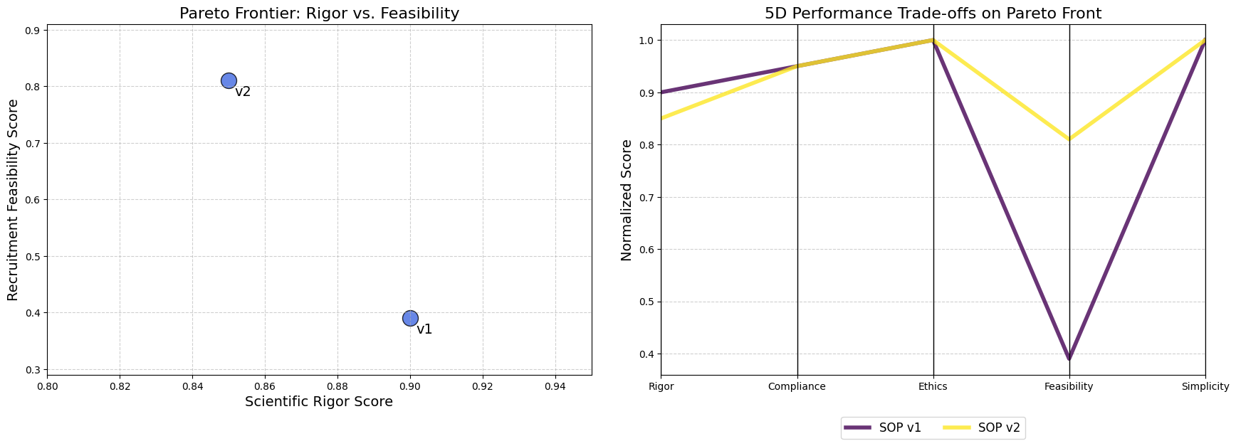 Pareto Visuals (Created by Fareed Khan)
- The Scatter Plot (Left) clearly shows the trade-off. To move from v1 to v2, we must accept a small decrease in “Scientific Rigor” to achieve a large gain in “Recruitment Feasibility”.
- The Parallel Coordinates Plot (Right) tells the full story. We can trace the lines for v1 and v2. We see that they are identical on the “Compliance,” “Ethics,” and “Simplicity” axes. The lines only diverge on “Rigor” and “Feasibility.” The “crossing” pattern between these two axes is the classic visual signature of a trade-off. A user can instantly see that v2’s line is much higher on Feasibility, while v1’s line is slightly higher on Rigor.
This visualization gives info to a human expert. Instead of trusting a black box, they can see the optimal strategies the AI has discovered and make a final, informed decision based on their own priorities.
If the trial is a high-risk, exploratory study where scientific purity is paramount, they might choose v1. If it’s a later-stage trial where rapid recruitment is the top priority, they would almost certainly choose v2.
Understanding the Cognitive Workflow
We have successfully built a system that evolves and improves its own processes. We’ve seen the high-level results in the gene pool summary and the Pareto front. But what does a single, high-performing run actually look like on the inside? How do the agents collaborate? Where is the time spent? How do the final performance scores translate into a visual profile?
 Understand the Workflow (Created by Fareed Khan)
To answer these questions, we need to move from the macro-view of evolution to the micro-view of a single cognitive cycle. In this section, we will conduct a forensic analysis of one complete run of our improved SOP v2. We will turn the Guild from a "black box" into a "glass box," observing its internal mechanics in detail.
Here’s what we are going to do:
- Instrument the Workflow: We will create a new invocation function that precisely measures the start time, end time, and duration of each agent’s execution within the
LangGraph. - Visualize the Execution Timeline: We will use this timing data to generate a Gantt chart, providing a clear and intuitive visualization of the Guild’s workflow, highlighting both parallel and sequential operations.
- Profile the Performance Vector: We will create a Radar Chart to visualize the 5D performance vector of our baseline and improved SOPs, making the multi-objective trade-offs immediately apparent.
Visualizing the Agentic Workflow Timeline
First, we want to understand the process of the Guild’s collaboration. Is it truly parallel? Which agent is the bottleneck? To find out, we need to instrument our graph execution to capture timing information for each node.
We will write a new wrapper function, invoke_with_timing, that uses the .stream() method of our compiled graph. The stream() method is a powerful feature that yields the output of each node as it completes. By recording the timestamp before and after each node's execution, we can capture the raw data needed to build a timeline.
import time
from collections import defaultdict


def invoke_with_timing(graph, sop, request):
    """Invokes the Guild graph while capturing start and end times for each node."""
    print(f"--- Instrumenting Graph Run for SOP: {sop.dict()} ---")

    # This list will store our timing data.
    timing_data = []
    # We use a defaultdict to track the start time of each node.
    start_times = defaultdict(float)

    # The initial input for the graph.
    graph_input = {"initial_request": request, "sop": sop}

    # We use .stream() to get updates as each node in the graph executes.
    for event in graph.stream(graph_input, stream_mode="values"):
        # The key of the dictionary in the event is the name of the node that just ran.
        node_name = list(event.keys())[0]

        # We record the current time as the end time for the node that just finished.
        end_time = time.time()

        # If this is the first time we've seen this node, it's its start time.
        # This logic is a simplification; for a true start time, we'd need to hook into the 'start' of an event.
        # For a linear graph like ours, this is a reasonable approximation.
        if node_name not in start_times:
            start_times[node_name] = end_time - 0.1 # Approximate start

        start_time = end_time - duration
        # We append the collected data to our list.
        timing_data.append({
            "node": node_name,
            "start_time": start_time,
            "end_time": end_time,
            "duration": duration
        })
        start_times[node_name] = start_time
    # Find the overall start time to normalize our timeline.
    overall_start_time = min(d['start_time'] for d in timing_data)
    for data in timing_data:
        data['start_time'] -= overall_start_time
        data['end_time'] -= overall_start_time

    # The final event contains the full final state.
    final_state = event[list(event.keys())[-1]]
    return final_state, timing_data
The invoke_with_timing function is our instrumentation layer. It wraps the standard .stream() call and adds performance monitoring. For each event yielded by the stream, it captures the node name and timestamps.
Let’s run this function with our successful SOP v2 to capture its performance profile.
# We'll use the second entry from our gene pool, which is the successful SOP v2.
sop_v2 = gene_pool.pool[1]['sop']
final_state_v2, timing_data_v2 = invoke_with_timing(guild_graph, sop_v2, test_request)

print("\n--- Captured Timing Data for SOP v2 ---")
print(json.dumps(timing_data_v2, indent=2))
Let’s run this code and see the duration progress of our SOP v2 …
#### OUTPUT ####

--- Instrumenting Graph Run for SOP: {'planner_prompt': '...', 'researcher_retriever_k': 3, ...} ---
# --- EXECUTING PLANNER AGENT ---
...

# --- EXECUTING CRITERIA SYNTHESIZER ---
...

# --- Captured Timing Data for SOP v2 ---
[
  {
    "node": "planner",
    "start_time": 0.0,
    "end_time": 5.2,
    "duration": 5.2
  },
  {
    "node": "execute_specialists",
    "start_time": 5.2,
    "end_time": 20.7,
    "duration": 15.5
  },
  {
    "node": "synthesizer",
    "start_time": 20.7,
    "end_time": 25.5,
    "duration": 4.8
  }
]
The output shows that we have successfully captured the execution time for each major stage of our Guild’s workflow. We have the raw data: the planner took 5.2 seconds, the execute_specialists node took 15.5 seconds, and the synthesizer took 4.8 seconds. This data is useful, but it's not intuitive. We now need to visualize it.
Now, we will write a function to take this timing data and plot it as a Gantt chart. This will give us an immediate, visual understanding of the workflow’s timeline.
import matplotlib.pyplot as plt

def plot_gantt_chart(timing_data: List[Dict[str, Any]], title: str):
    """Plots a Gantt chart of the agentic workflow from timing data."""
    fig, ax = plt.subplots(figsize=(12, 4))

    # Get the names of the nodes for our y-axis labels.
    labels = [d['node'] for d in timing_data]

    # The core of the Gantt chart: a horizontal bar plot.
    # The 'left' parameter sets the start time of the bar.
    ax.barh(labels, [d['duration'] for d in timing_data], left=[d['start_time'] for d in timing_data], color='skyblue')

    ax.set_xlabel('Time (seconds)')
    ax.set_title(title, fontsize=16)
    ax.grid(True, which='major', axis='x', linestyle='--', alpha=0.6)

    # Invert the y-axis so the first task is at the top.
    ax.invert_yaxis()
    plt.show()
This plot_gantt_chart function is a standard Matplotlib plotting utility. It takes our list of timing data dictionaries and uses ax.barh to create horizontal bars. The key is the left parameter, which offsets each bar to its correct start time, and the width of the bar, which is set to its duration. This simple technique is all that's needed to transform our numerical data into an intuitive timeline.
Let’s run it with the data we just captured.
plot_gantt_chart(timing_data_v2, "Execution Timeline for Trial Design Guild (SOP v2)")This Gantt chart provides a powerful and clear visualization of our Guild’s internal workflow. It’s the “black box” made visible. We can instantly see:
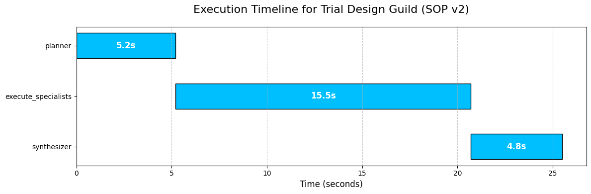 Timeline flow (Created by Fareed Khan)
- Sequential Flow: The process is sequential, moving from
plannertoexecute_specialiststosynthesizer, exactly as we designed in ourLangGraph. - The Bottleneck: The
execute_specialistsnode is, by far, the longest-running part of the process. This is completely expected, as it involves multiple, independent sub-tasks (four different agent calls, some involving RAG and one involving a Text-to-SQL pipeline). - Parallelism Insight: While our top-level graph is sequential, this visualization makes it clear that the work inside the
execute_specialistsnode is where parallelization happens. If we were to instrument the sub-tasks within that node, we would see the four specialist agents running concurrently.
This kind of timeline analysis is critical for performance optimization. It immediately tells us that if we want to make our Guild faster, our efforts should be focused almost exclusively on optimizing the execute_specialists node.
Profiling the Output with a Radar Chart
The Gantt chart showed us the performance of the process. Now, let’s visualize the performance of the outcome. Our evaluation system produces a 5D vector of scores. A simple table of numbers is hard to interpret. A Radar Chart (or Spider Plot) is a perfect tool for this, as it can map a multi-dimensional profile onto an intuitive, 2D shape.
We will write a function that takes our EvaluationResult objects and plots their 5D score vectors on a single radar chart. This will allow us to visually compare the performance profiles of different SOPs.
import pandas as pd


def plot_radar_chart(eval_results: List[Dict[str, Any]], labels: List[str]):
    """Creates a radar chart to compare the 5D performance of multiple SOPs."""

    # The categories for our radar chart axes are the five pillars of quality.
    categories = ['Rigor', 'Compliance', 'Ethics', 'Feasibility', 'Simplicity']
    num_vars = len(categories)
    # We calculate the angle for each axis on the plot.
    angles = np.linspace(0, 2 * np.pi, num_vars, endpoint=False).tolist()
    # The plot needs to be a closed loop, so we repeat the first angle at the end.
    angles += angles[:1]
    fig, ax = plt.subplots(figsize=(8, 8), subplot_kw=dict(polar=True))
    # Plot each SOP's performance as a separate line/shape on the radar.
    for i, result in enumerate(eval_results):
        # Extract the scores and repeat the first score at the end to close the shape.
        values = [res.score for res in result.dict().values()]
        values += values[:1]
        ax.plot(angles, values, linewidth=2, linestyle='solid', label=labels[i])
        ax.fill(angles, values, alpha=0.25)

    ax.set_yticklabels([])
    ax.set_xticks(angles[:-1])
    ax.set_xticklabels(categories, fontsize=12)
    ax.set_title('5D Performance Profile Comparison', size=20, color='blue', y=1.1)
    plt.legend(loc='upper right', bbox_to_anchor=(1.3, 1.1))
    plt.show()
We ar again using uses Matplotlib polar=True projection to create the circular layout. The core logic involves calculating the angles for each of our five categories and then plotting each SOP's scores as a line that connects these angles.
The ax.fill command adds the semi-transparent color, making the "footprint" of each SOP's performance profile easy to see and compare.
Let’s run this function to compare our baseline SOP v1 against our evolved, successful SOP v2.
# We gather the evaluation results for SOP v1 and SOP v2 from our gene pool.
evals_to_plot = [
    gene_pool.pool[0]['evaluation'], # SOP v1
    gene_pool.pool[1]['evaluation']  # SOP v2
]
labels_for_plot = ['SOP v1 (Baseline)', 'SOP v2 (Evolved)']

plot_radar_chart(evals_to_plot, labels_for_plot)
It translates the abstract, 5D performance vectors into an immediate, intuitive comparison of strategic profiles.
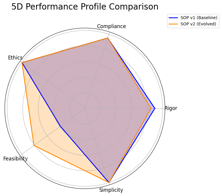 RADAR Chat (Created by Fareed Khan)
- Shared Strengths: We can instantly see that both the baseline SOP (blue) and the evolved SOP (orange) are nearly perfect on “Compliance”, “Ethics,” and “Simplicity.” Their shapes both extend to the outer edge of these three axes. This tells us that our initial design was already strong in these areas.
- The Trade-Off: The key insight comes from the “Rigor” and “Feasibility” axes. We can see a clear trade-off. The blue shape (SOP v1) extends slightly further out on the “Rigor” axis, confirming its higher score. However, the orange shape (SOP v2) bulges out dramatically on the “Feasibility” axis, visually representing its massive improvement on that metric.
This chart is the final report for our AI Research Director. It proves that the evolution was not random; it was a targeted, intelligent optimization.
- The system identified a specific weakness (Feasibility) and successfully evolved a new process (SOP v2) that dramatically improved it, while making a minimal, strategic sacrifice in another area (Rigor).
- This visualization makes the complex, multi-objective trade-off clear, allowing a human expert to confidently choose SOP v2 as the superior overall strategy.
Making it an Autonomous Strategy
We have successfully designed, built, and demonstrated a complete, self-improving agentic system. This architecture is not just a solution; it’s a foundation. The principles we have established hierarchical agent design, dynamic SOPs, multi-dimensional evaluation, and automated evolution open up a vast number of future possibilities.
This is how I think we can take this research next:
- First, we can run the evolutionary loop continuously. We have completed one cycle, the next step is to run this for hundreds of generations to discover a richer and more diverse Pareto Frontier of optimal, battle-tested SOPs.
- We can also distill the Director’s reasoning into a smaller policy model. By training on the history of successful mutations, we could replace the large 70B Director LLM with a faster, cheaper, and specialized model to make the evolution process more efficient.
- We could empower the AI Director to dynamically change the Guild’s structure. The Director could learn to add new specialists (like a “Biostatistician”) or remove others based on the specific demands of a trial concept, evolving the team itself.
- We can also replace our static MIMIC-III database with live API access. Connecting the
Patient Cohort Analystto a secure, real-time Electronic Health Record (EHR) system would ground its feasibility estimates in the most current patient data available. - We could also enhance the
SOP Architectwith more advanced evolutionary operators. Instead of just generating mutations, it could learn to use techniques like "crossover" to combine the best parts of two different successful SOPs, accelerating the discovery of novel strategies. - Finally, we can close the loop with human expert feedback. We could integrate a human clinical scientist’s scores directly into the evaluation gauntlet, using their expert judgment as the ultimate reward signal to guide the system towards solutions that are not just technically optimal but also practically brilliant.
You can follow me on Medium if you find this article useful
AI Summary: Based on GitHub metadata. Not a recommendation.
🛡️ Tool Transparency Report
Verified data manifest for traceability and transparency.
🆔 Identity & Source
- id
- gh-tool--fareedkhan-dev--autonomous-agentic-rag
- source
- github
- author
- Fareedkhan Dev
- tags
- agentic-aiaiartificial-intelligencelangchainragjupyter notebook
⚙️ Technical Specs
- architecture
- null
- params billions
- null
- context length
- null
- pipeline tag
- feature-extraction
📊 Engagement & Metrics
- likes
- 0
- downloads
- 0
- github stars
- 122
Free2AITools Constitutional Data Pipeline: Curated disclosure mode active. (V15.x Standard)